Generate Synthetic Sensor Data for Localization Using Unreal Engine

Set Up Vehicle Parameters

Load the haul truck rigid body tree model, and compute the geometric parameters required for ground following and sensor placement.

[haultruck,importInfo] = loadvehicle("haultruck");
wheelBase = importInfo.WheelBase;
trackWidth = importInfo.RearTrackWidth;
wheelRadius = importInfo.WheelRadius;

The rear axle frame sits midway between the rear wheels, with the same orientation as the rear-left wheel frame.

q = homeConfiguration(haultruck);
rearAxlePose = getTransform(haultruck,q,"rear_axle_center");
show(haultruck,FrameSize=2)
title("Haul Truck Model")
axis auto

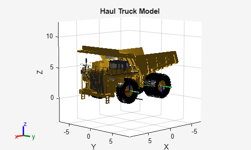
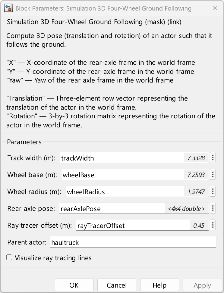
To ensure the vehicle snaps to the ground at its initial 2D pose (x, y, theta) and the emitted ray intersects the ground rather than the vehicle body, offset the ray tracer axially by 0.45 meters. This value has been determined through trial and error.

initXYZ = [-30 0 10];
initTheta = 0;
rayTracerOffset = 0.45;

The camera shares the orientation of the body frame, offset by 1 meter in the body frame positive-x direction.

rbase_cam = tform2trvec(getTransform(haultruck,q,"body")*trvec2tform([1 0 0]));

Open Simulink Model

The model consists of these areas and blocks:

mdl = "IMUAndCameraSensorsOnHaulTruckInSim3d";
open_system(mdl)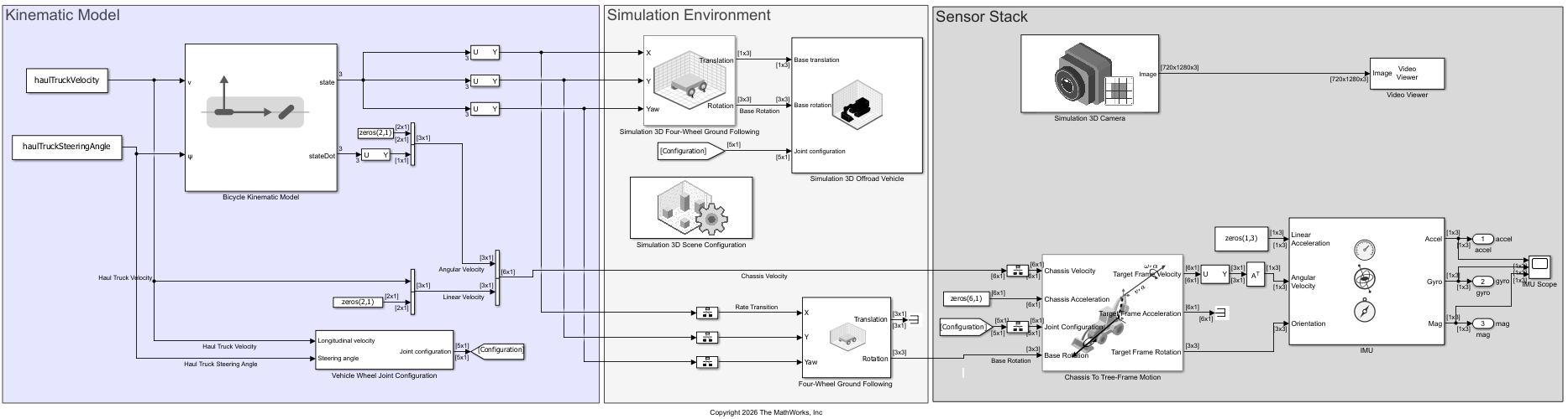

Configure Kinematic Model

The Kinematic Model area of the model drives the haul truck along a path using a Bicycle Kinematic Model block. The block accepts speed and steering angle inputs and outputs the vehicle pose.

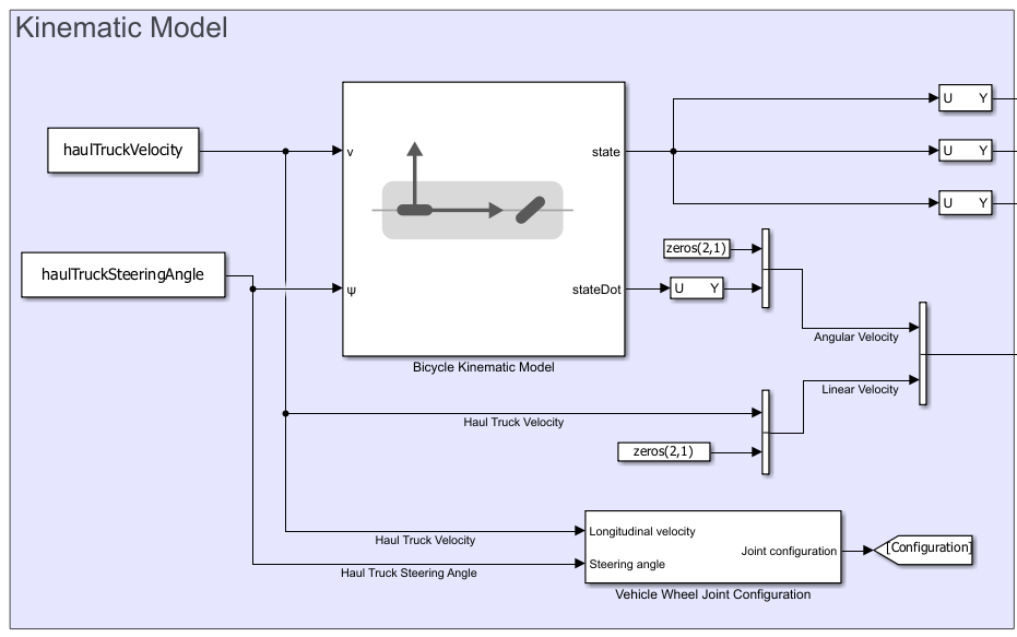
Load a recorded trajectory, represented as a timeseries of velocities and steering angles. You can also replace this trajectory with live data.

load("exampleHelperHaulTruckTrajectory.mat")

Configure Simulation Environment

The Simulation Environment area configures the 3D scene and adapts the vehicle pose to the terrain. The Simulation 3D Scene Configuration block connects MATLAB® to the Unreal Engine rendering environment.

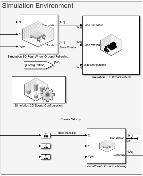
The example uses the Construction site scene as the 3D simulation environment.

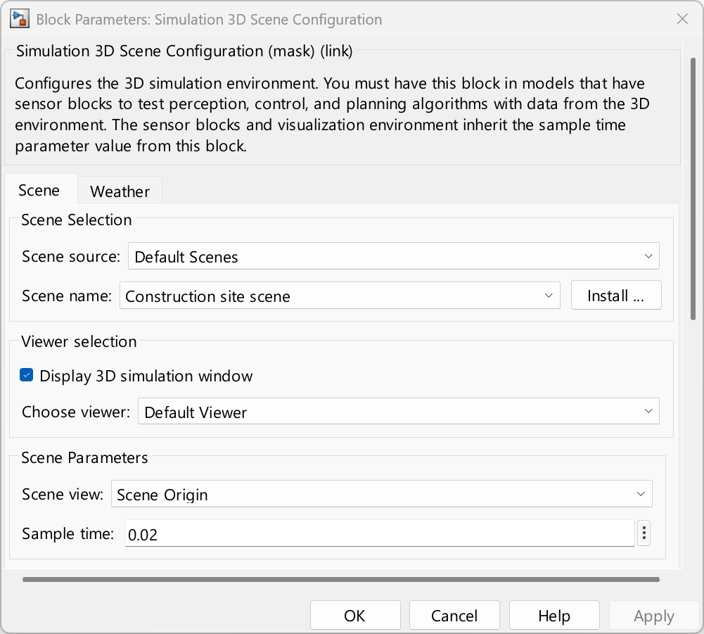
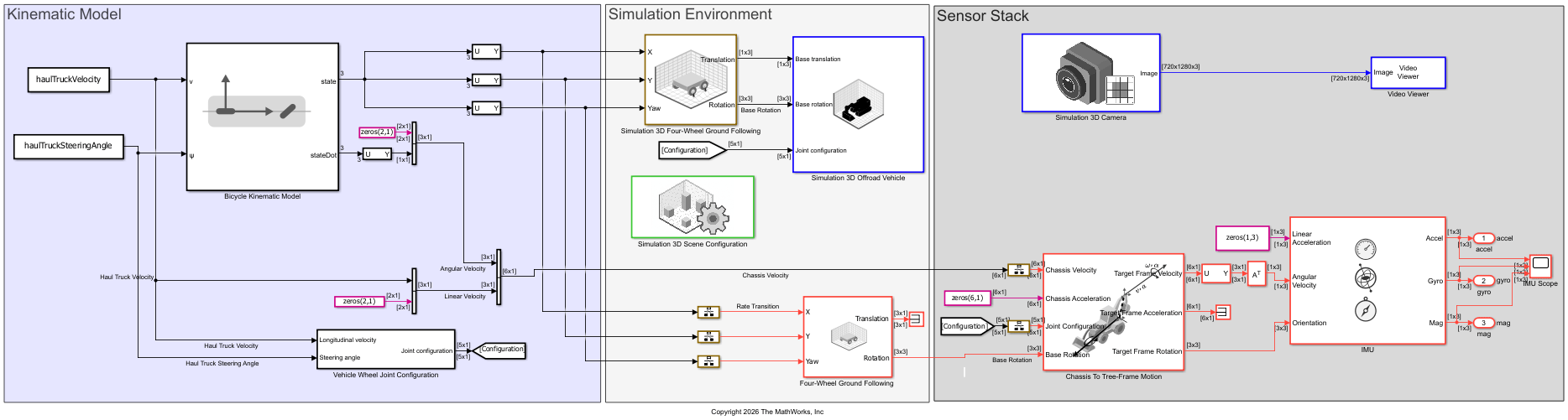
To transform the 2D pose of the vehicle (x, y, yaw) into a ground-following 3D pose, use the Simulation 3D Four-Wheel Ground Following block. The block emits four ray tracers that detect the ground surface, snapping the vehicle to the terrain based on the vehicle parameters.

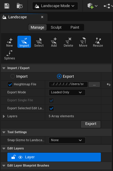
To collect IMU data at a faster rate than the Simulation 3D block allows, the model uses an additional Four-Wheel Ground Following block that operates on a heightmap exported from Unreal Engine. To export the terrain, follow these steps:

In the Unreal Editor, enter Landscape mode, select the Import tool under Manage mode, and click Export. Enable the Heightmap File checkbox, choose a file name, and save as a 16-bit grayscale PNG. Adjust settings as needed (see Unreal Landscape Export Settings documentation), then click Export.

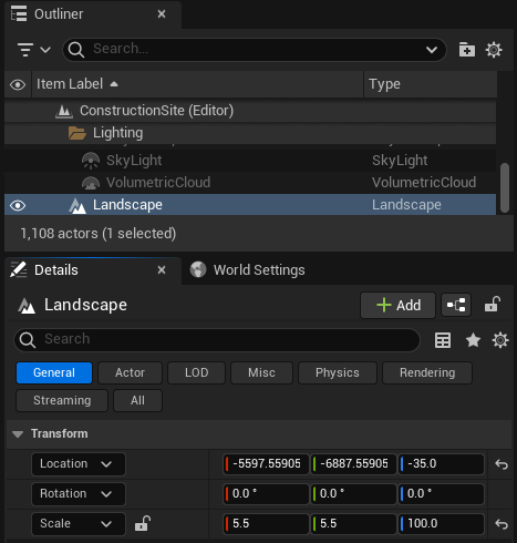
Note down the Translation, Rotation, and Scale parameters of the Landscape object. These are visible in the General tab when the Landscape actor is selected.

Use the exported PNG file with the Four-Wheel Ground Following Simulink block. Enter the noted parameters into the block's Terrain mask parameters. Convert from centimeters (Unreal) to meters (MATLAB).

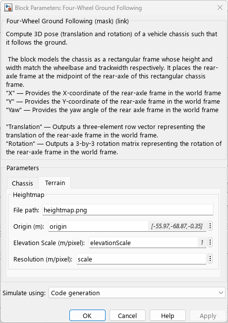
For this example, the Unreal Landscape parameters and their converted values are:

% Landscape parameters from Unreal Editor (in centimeters)
unrealTranslation = [-5597, -6887, -35];
unrealScale = [5.5, 5.5, 100];

% Convert from centimeters to meters for the block
origin = unrealTranslation / 100;            % [-55.97, -68.87, -0.35] m
scale = unrealScale(1:2) / 100;              % [0.055, 0.055] m
elevationScale = unrealScale(3) / 100;       % 1.0 m

The following image highlights the rate regions in the model — the Simulation 3D Camera block captures images at 10 Hz (blue) and the Four-Wheel Ground Following block provides terrain data for the IMU at 100 Hz (red).

Configure Sensor Stack

The Sensor Stack area generates sensor data for a camera and an IMU. The Chassis To Tree-Frame Motion block computes body-frame linear velocity, acceleration, and orientation, the IMU (Navigation Toolbox) block produces accelerometer, gyroscope, and magnetometer readings, and the Simulation 3D Camera block captures monocular RGB images.

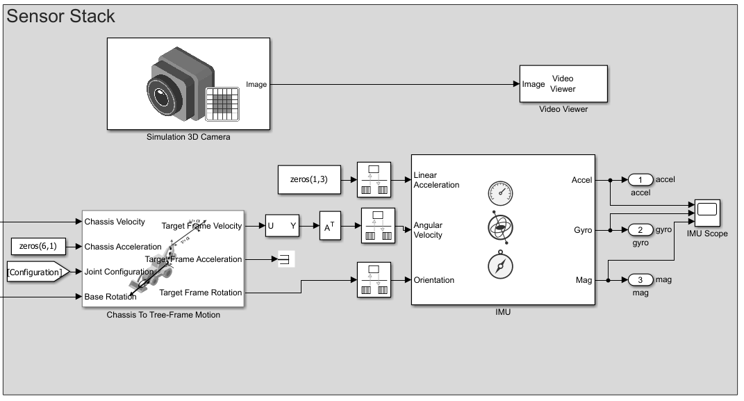
You can place the IMU on any frame of the rigid body tree by setting the TargetFrameName parameter. The block transforms chassis-frame velocity to the target frame using the same approach as the transformMotion function, and accounts for the joint configuration of the rigid body tree. For more information on the transformation approach, see Motion Quantities Used in transformMotion.

get_param(mdl+"/Chassis To Tree-Frame Motion","TargetFrameName")

ans = 
'body'

Simulate Model

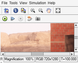
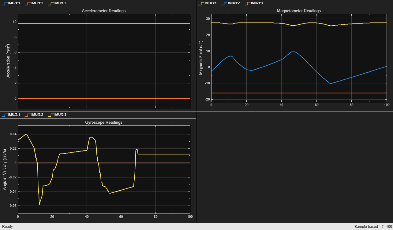
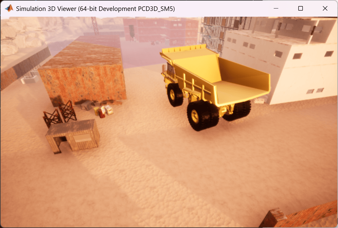
When you simulate the model, the Unreal Engine rendering window opens and shows the haul truck moving through the construction site scene. The IMU block generates sensor readings at the configured sample rate, and the camera captures images at each simulation time step.

out = sim(mdl);

Visualize IMU Sensor Data

Extract and plot the accelerometer, gyroscope, and magnetometer data from the simulation output. These signals represent what a physical IMU mounted on the vehicle body would measure.

accelData = out.yout.get("accel").Values;
gyroData = out.yout.get("gyro").Values;
magData = out.yout.get("mag").Values;

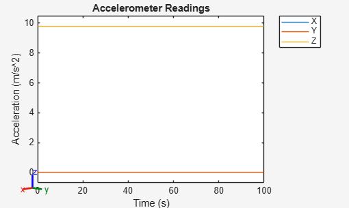
Plot the accelerometer readings. The z-axis shows the gravity component modulated by vehicle pitch and roll as it traverses uneven terrain.

plot(accelData)
title("Accelerometer Readings")
xlabel("Time (s)")
ylabel("Acceleration (m/s^2)")
ylim padded
legend("X","Y","Z")

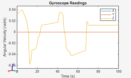
Plot the gyroscope readings. The angular velocity changes correspond to steering maneuvers and terrain-induced rotations.

plot(gyroData)
title("Gyroscope Readings")
xlabel("Time (s)")
ylabel("Angular Velocity (rad/s)")
ylim padded
legend("X","Y","Z")

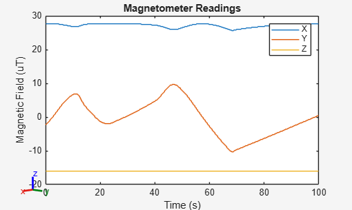
Plot the magnetometer readings.

plot(magData)
title("Magnetometer Readings")
ylabel("Magnetic Field (uT)")
xlabel("Time (s)")
ylim padded
legend("X","Y","Z")