dlstft
Deep learning short-time Fourier transform
Description
y = dlstft(x)x. dlstft requires Deep Learning Toolbox™.
y = dlstft(___,Name,Value)'DataFormat','CBT' specifies the data format of
x as CBT.
Examples
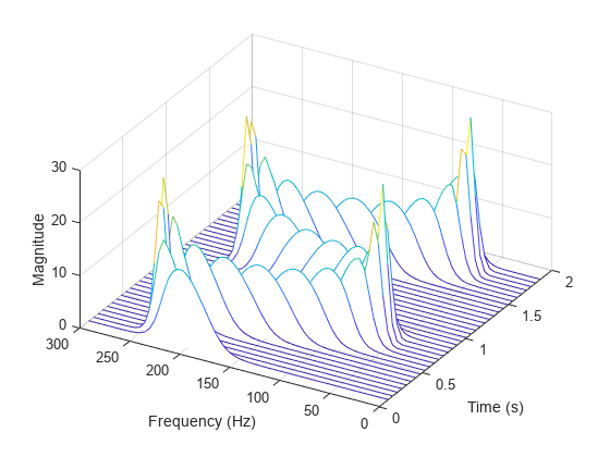
Generate a signal sampled at 600 Hz for 2 seconds. The signal consists of a chirp with sinusoidally varying frequency content.
fs = 6e2;
t = 0:1/fs:2;
x = vco(sin(2*pi*t),[0.1 0.4]*fs,fs);
Store the signal in an unformatted deep learning array. Compute the short-time Fourier transform of the signal. Input the sample time as a duration scalar. (Alternatively, input the sample rate as a numeric scalar.) Specify that the input array is in 'CTB' format.
dlx = dlarray(x);

[y,f,t] = dlstft(dlx,seconds(1/fs),'DataFormat','CTB');
Convert the outputs to numeric arrays. Compute the magnitude of the short-time Fourier transform and display it as a waterfall plot.
y = extractdata(y);
f = extractdata(f);
t = seconds(t);

waterfall(f,t,squeeze(abs(y))')

ax = gca;
ax.XDir = 'reverse';
view(30,45)

ylabel('Time (s)')
xlabel('Frequency (Hz)')
zlabel('Magnitude')

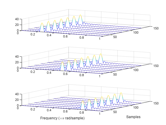
Generate a 3-by-160(-by-1) array containing one batch of a three-channel, 160-sample sinusoidal signal. The normalized sinusoid frequencies are rad/sample, rad/sample, and rad/sample. Save the signal as a dlarray, specifying the dimensions in order. dlarray permutes the array dimensions to the 'CBT' shape expected by a deep learning network. Display the array dimension sizes.
x = dlarray(cos(pi.*(1:3)'/4*(0:159)),'CTB');
[nchan,nbtch,nsamp] = size(x)
nchan = 3
nbtch =
1
nsamp =
160
Compute the deep learning short-time Fourier transform of the signal. Specify a 64-sample rectangular window and an FFT length of 1024.
[y,f,t] = dlstft(x,'Window',rectwin(64),'FFTLength',1024);
dlstft computes the transform along the 'T' dimension. The output array is in 'SCBT' format. The 'S' dimension corresponds to frequency in the short-time Fourier transform. Extract the data from the deep learning array.
y = extractdata(y);
f = extractdata(f);
t = extractdata(t);
Compute the magnitude of the short-time Fourier transform. Plot the magnitude separately for each channel in a waterfall plot.
z = abs(squeeze(y));

for kj = 1:nchan
    subplot(nchan,1,kj)
    waterfall(f/pi,t,squeeze(z(:,kj,:))')
    view(30,45)
end

xlabel('Frequency (\times\pi rad/sample)')
ylabel('Samples')

Input Arguments
Input array, specified as an unformatted dlarray (Deep Learning Toolbox) object,
a formatted dlarray object in 'CBT' format, or a
numeric array. If x is an unformatted dlarray or a
numeric array, you must specify the 'DataFormat' as some
permutation of 'CBT'.
Example: dlarray(cos(pi./[4;2]*(0:159)),'CTB') and
dlarray(cos(pi./[4;2]*(0:159))','TCB') both specify one batch
observation of a two-channel sinusoid in the 'CBT'
format.
Sample rate, specified as a positive numeric scalar.
Sample time, specified as duration scalar. Specifying
ts is equivalent to setting a sample rate fs =
1/ts.
Example: seconds(1) is a duration scalar
representing a 1-second time difference between consecutive signal
samples.
Name-Value Arguments
Specify optional pairs of arguments as
Name1=Value1,...,NameN=ValueN, where Name is
the argument name and Value is the corresponding value.
Name-value arguments must appear after other arguments, but the order of the
pairs does not matter.
Before R2021a, use commas to separate each name and value, and enclose
Name in quotes.
Example: 'Window',hamming(100),'OverlapLength',50,'FFTLength',128
windows the data using a 100-sample Hamming window, with 50 samples of overlap between
adjoining segments and a 128-point FFT.
Input data format, specified as a character vector or string scalar. This argument
is valid only if x is unformatted.
Each character in this argument must be one of these labels:
C— ChannelB— Batch observationsT— Time
The dlstft function accepts any permutation of
'CBT'. You can specify at most one of each of the
C, B, and T labels.
Each element of the argument labels the matching dimension of
x. If the argument is not in the listed order
('C' followed by 'B' and so on), then
dlstft implicitly permutes both the argument and the data
to match the order, but without changing how the data is stored.
Example: 'CBT'
Spectral window, specified as a vector. If you do not specify the window or
specify it as empty, the function uses a Hann window of length 128. The length of
'Window' must be greater than or equal to 2.
For a list of available windows, see Windows.
Example: hann(N+1) and
(1-cos(2*pi*(0:N)'/N))/2 both specify a Hann window of length
N + 1.
Data Types: double | single
Number of overlapped samples, specified as a nonnegative integer smaller than the
length of 'Window'. If you omit
'OverlapLength' or specify it as empty, it is set to the
largest integer less than 75% of the window length, which is 96 samples for the
default Hann window.
Data Types: double | single
Number of DFT points, specified as a positive integer. The value must be greater than or equal to the window length. If the length of the input signal is less than the DFT length, the data is padded with zeros.
Data Types: double | single
Output Arguments
Short-time Fourier transform, returned as a formatted or unformatted dlarray (Deep Learning Toolbox)
object.
If
xis a formatteddlarray, thenyis an'SCBT'formatteddlarrayobject. The'S'dimension corresponds to frequency in the short-time Fourier transform.If
xis an unformatteddlarrayor a numeric array, thenyis an unformatteddlarrayobject. The dimension order inyis'SCBT'.
If no time information is specified, then the STFT is computed over the Nyquist
range [0, π] if 'FFTLength' is even and over [0, π) if 'FFTLength' is odd. If you specify time
information, then the intervals are [0, fs/2] and [0, fs/2), respectively, where fs is
the effective sample rate.
Frequencies at which the deep learning STFT is computed, returned as a
dlarray object.
If the input array does not contain time information, then the frequencies are in normalized units of rad/sample.
If the input array contains time information, then
fcontains frequencies expressed in Hz.
Times at which the deep learning STFT is computed, returned as a
dlarray object or a duration array.
If you do not specify time information, then
tcontains sample numbers.If you specify a sample rate, then
tcontains time values in seconds.If you specify a sample time, then
tis adurationarray with the same time format asx.
More About
The short-time Fourier transform (STFT) is used to analyze how the frequency content of a nonstationary signal changes over time. The magnitude squared of the STFT is known as the spectrogram time-frequency representation of the signal. For more information about the spectrogram and how to compute it using Signal Processing Toolbox™ functions, see Spectrogram Computation with Signal Processing Toolbox.
The STFT of a signal is computed by sliding an analysis window g(n) of length M over the signal and calculating the discrete Fourier transform (DFT) of each segment of windowed data. The window hops over the original signal at intervals of R samples, equivalent to L = M – R samples of overlap between adjoining segments. Most window functions taper off at the edges to avoid spectral ringing. The DFT of each windowed segment is added to a complex-valued matrix that contains the magnitude and phase for each point in time and frequency. The STFT matrix has
columns, where Nx is the length of the signal x(n) and the ⌊⌋ symbols denote the floor function. The number of rows in the matrix equals NDFT, the number of DFT points, for centered and two-sided transforms and an odd number close to NDFT/2 for one-sided transforms of real-valued signals.
The mth column of the STFT matrix contains the DFT of the windowed data centered about time mR:
Extended Capabilities
C/C++ Code Generation
Generate C and C++ code using MATLAB® Coder™. (since R2025a)
GPU Code Generation
Generate CUDA® code for NVIDIA® GPUs using GPU Coder™. (since R2025a)
This function fully supports GPU arrays. For more information, see Run MATLAB Functions on a GPU (Parallel Computing Toolbox).
Version History
Introduced in R2021aThe dlstft function supports:
C/C++ code generation. You must have MATLAB® Coder™ to generate C/C++ code.
Code generation for NVIDIA® GPUs. You must have GPU Coder™ to generate GPU code.
Starting in R2023b, dlstft combines the real and imaginary
parts of the STFT into a single output argument. Previously, the function returned the real
part of the transform as the first output argument and the imaginary part as the second.
Starting this release, the function returns as second and third output arguments the
frequencies and times at which the STFT is computed, respectively. Function calls with four
output arguments error out.
| Original Code in R2023a or Earlier | Result | Updated Code in R2023b |
|---|---|---|
[yr,yi] = dlstft(x); | Runs, but the second output argument has a different interpretation | y = dlstft(x); yr = real(y); yi = imag(y); |
[yr,yi,f,t] = dlstft(x); | Errors | [y,f,t] = dlstft(x); yr = real(y); yi = imag(y); |
See Also
Objects
stftLayer|istftLayer|dlarray(Deep Learning Toolbox)
Functions
dlistft|stft|istft|stftmag2sig
Topics
- Spoken Digit Recognition with Custom Log Spectrogram Layer and Deep Learning
- List of Functions with dlarray Support (Deep Learning Toolbox)
- Code Generation for dlarray (MATLAB Coder)
- Code Generation for dlarray (GPU Coder)
MATLAB Command
You clicked a link that corresponds to this MATLAB command:
Run the command by entering it in the MATLAB Command Window. Web browsers do not support MATLAB commands.
选择网站
选择网站以获取翻译的可用内容,以及查看当地活动和优惠。根据您的位置,我们建议您选择:。
您也可以从以下列表中选择网站:
如何获得最佳网站性能
选择中国网站(中文或英文)以获得最佳网站性能。其他 MathWorks 国家/地区网站并未针对您所在位置的访问进行优化。
美洲
- América Latina (Español)
- Canada (English)
- United States (English)
欧洲
- Belgium (English)
- Denmark (English)
- Deutschland (Deutsch)
- España (Español)
- Finland (English)
- France (Français)
- Ireland (English)
- Italia (Italiano)
- Luxembourg (English)
- Netherlands (English)
- Norway (English)
- Österreich (Deutsch)
- Portugal (English)
- Sweden (English)
- Switzerland
- United Kingdom (English)