stft

s = stft(x,fs) 使用采样率 fs 返回 x 的 STFT。

s = stft(x,ts) 使用采样时间 ts 返回 x 的 STFT。

s = stft(___,Name=Value) 使用名称-值参量指定附加选项。选项包括 FFT 窗和长度。这些参量可以添加到上述任一输入语法。

[s,f] = stft(___) 返回在其上计算 STFT 的频率 f。

[s,f,t] = stft(___) 返回在其上计算 STFT 的时间。

不带输出参量的 stft(___) 在当前图窗窗口中以分贝为单位绘制 STFT 的幅值平方。

短时傅里叶变换

生成频率呈正弦变化的啁啾。信号以 10 kHz 频率进行 2 秒采样。

fs = 10e3;
t = 0:1/fs:2;
x = vco(sin(2*pi*t),[0.1 0.4]*fs,fs);

计算啁啾的短时傅里叶变换。将信号分成长度为 256 个采样的段，并使用形状参数 β = 5 的凯塞窗对每个段加窗。指定相邻段之间有 220 个采样的重叠，并指定 DFT 长度为 512。输出在其上计算 STFT 的频率和时间值。

[s,f,t] = stft(x,fs,Window=kaiser(256,5),OverlapLength=220,FFTLength=512);

STFT 的幅值平方也称为频谱图。以分贝为单位绘制频谱图。指定一个跨 60 dB 的颜色图，其最后颜色对应频谱图的最大值。

sdb = mag2db(abs(s));
mesh(t,f/1000,sdb);

cc = max(sdb(:))+[-60 0];
ax = gca;
ax.CLim = cc;
view(2)
colorbar

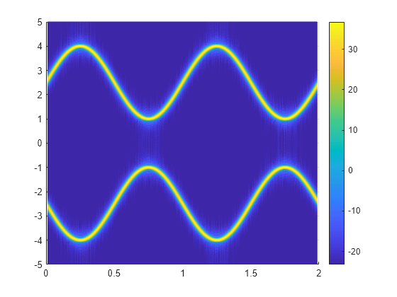
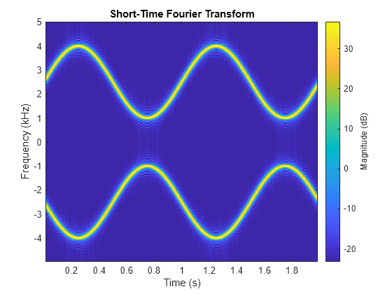
Figure contains an axes object. The axes object contains an object of type surface.

通过调用不带输出参量的 stft 函数获得相同的图。

stft(x,fs,Window=kaiser(256,5),OverlapLength=220,FFTLength=512)

Figure contains an axes object. The axes object with title Short-Time Fourier Transform, xlabel Time (s), ylabel Frequency (kHz) contains an object of type image.

二次啁啾的 STFT

生成以 1 kHz 进行 2 秒采样的二次啁啾。瞬时频率在 $t = 0$ 处为 100 Hz，并在 $t = 1$ 秒处超出 200 Hz。

ts = 0:1/1e3:2;

f0 = 100;
f1 = 200;

x = chirp(ts,f0,1,f1,"quadratic",[],"concave");

计算并显示持续 1 毫秒的二次啁啾的 STFT。

d = seconds(1e-3);
win = hamming(100,"periodic");

stft(x,d,Window=win,OverlapLength=98,FFTLength=128);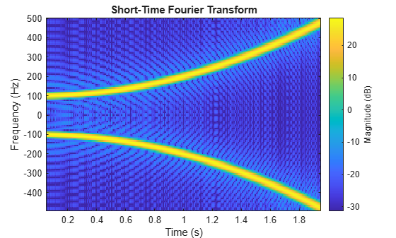

Figure contains an axes object. The axes object with title Short-Time Fourier Transform, xlabel Time (s), ylabel Frequency (Hz) contains an object of type image.

比较 `spectrogram` 和 `stft` 函数

生成一个由在 1.4 kHz 下采样 2 秒的啁啾组成的信号。在测量时间内，啁啾的频率从 600 Hz 线性增加到 100 Hz。

fs = 1400;
x = chirp(0:1/fs:2,600,2,100);

stft 默认值

使用 spectrogram 和 stft 函数计算信号的 STFT。使用 stft 函数的默认值：

将信号分成若干长度为 128 个采样的段，并使用周期性汉宁窗对每个段加窗。
指定相邻段之间有 96 个采样的重叠。此长度等效于窗长度的 75%。
指定 128 个 DFT 点并将 STFT 中心设在零频率处，频率以赫兹为单位表示。

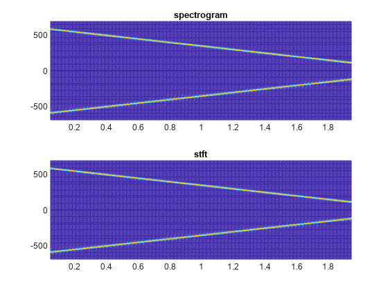
验证两个结果是否相等。

M = 128;
g = hann(M,"periodic");
L = 0.75*M;
Ndft = 128;

[sp,fp,tp] = spectrogram(x,g,L,Ndft,fs,"centered");

[s,f,t] = stft(x,fs);

dff = max(max(abs(sp-s)))

dff = 
0

使用 mesh 函数绘制两个输出。

nexttile
mesh(tp,fp,abs(sp).^2)
title("spectrogram")
view(2), axis tight

nexttile
mesh(t,f,abs(s).^2)
title("stft")
view(2), axis tight

Figure contains 2 axes objects. Axes object 1 with title spectrogram contains an object of type surface. Axes object 2 with title stft contains an object of type surface.

spectrogram 默认值

使用 spectrogram 函数的默认值重复计算：

将信号分成长度为 $M = ⌊ N_{x} / 4.5 ⌋$ 的段，其中 $N_{x}$ 是信号的长度。使用汉明窗对每个段加窗。
指定段之间有 50% 的重叠。
为了计算 FFT，请使用 $\max (256, 2^{⌈ \log_{2} M ⌉})$ 个点。仅计算正归一化频率的频谱图。

M = floor(length(x)/4.5);
g = hamming(M);
L = floor(M/2);
Ndft = max(256,2^nextpow2(M));

[sx,fx,tx] = spectrogram(x);

[st,ft,tt] = stft(x,Window=g,OverlapLength=L, ...
    FFTLength=Ndft,FrequencyRange="onesided");

dff = max(max(sx-st))

dff = 
0

使用 waterplot 函数绘制两个输出。在这两种情况下都将频率轴除以 $π$ 。对于 stft 输出，将采样数除以有效采样率 $2 π$ 。

figure
nexttile
waterplot(sx,fx/pi,tx)
title("spectrogram")

nexttile
waterplot(st,ft/pi,tt/(2*pi))
title("stft")

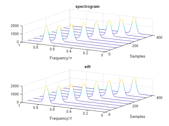
$Figure contains 2 axes objects. Axes object 1 with title spectrogram, xlabel Frequency/\pi, ylabel Samples contains an object of type patch. Axes object 2 with title stft, xlabel Frequency/\pi, ylabel Samples contains an object of type patch.$

function waterplot(s,f,t)
% Waterfall plot of spectrogram
    waterfall(f,t,abs(s)'.^2)
    set(gca,XDir="reverse",View=[30 50])
    xlabel("Frequency/\pi")
    ylabel("Samples")
end

STFT 频率范围

生成一个信号，其采样率为 5 kHz，采样时间持续 4 秒。信号由一组持续时间递减的脉冲组成，各脉冲由振幅振荡和频率波动且呈递增趋势的区域分隔。绘制信号。

fs = 5000;
t = 0:1/fs:4-1/fs;

x = besselj(0,600*(sin(2*pi*(t+1).^3/30).^5));

plot(t,x)

Figure contains an axes object. The axes object contains an object of type line.

计算信号的单边、双边和居中短时傅里叶变换。在所有情况下，使用形状因子为 $β = 10$ 的长度为 202 个采样的凯塞窗对信号段加窗。显示用于计算每个变换的频率范围。

rngs = ["onesided" "twosided" "centered"];

for kj = 1:length(rngs)
    
    opts = {"Window",kaiser(202,10),"FrequencyRange",rngs(kj)};

    [~,f] = stft(x,fs,opts{:});
    subplot(length(rngs),1,kj)
    stft(x,fs,opts{:})
    title(sprintf('''%s'': [%5.3f, %5.3f] kHz',rngs(kj),[f(1) f(end)]/1000))

end

重复计算，但现在将凯塞窗的长度更改为奇数 203。"twosided" 频率区间不变。其他两个频率区间在高端变为开放。

for kj = 1:length(rngs)
    
    opts = {"Window",kaiser(203,10),"FrequencyRange",rngs(kj)};

    [~,f] = stft(x,fs,opts{:});
    subplot(length(rngs),1,kj)
    stft(x,fs,opts{:})
    title(sprintf('''%s'': [%5.3f, %5.3f] kHz',rngs(kj),[f(1) f(end)]/1000))

end

多通道信号的 STFT

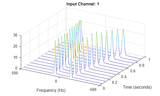
生成一个三通道信号，该信号由在 1 kHz 下采样一秒的三个不同啁啾组成。

第一个通道由凹二次啁啾组成，瞬时频率在 t = 0 处为 100 Hz，在 t = 1 秒处超出 300 Hz。其初始相位等于 45 度。
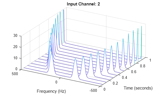
第二个通道由凸二次啁啾组成，瞬时频率在 t = 0 处为 100 Hz，在 t = 1 秒处超出 500 Hz。
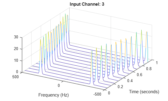
第三个通道由对数啁啾组成，瞬时频率在 t = 0 处为 300 Hz，在 t = 1 秒处超出 500 Hz。

使用长度为 128 的周期性汉明窗和 50 个采样的重叠长度计算多通道信号的 STFT。

fs = 1e3;
t = 0:1/fs:1-1/fs;

x = [chirp(t,100,1,300,"quadratic",45,"concave");
      chirp(t,100,1,500,"quadratic",[],"convex");
      chirp(t,300,1,500,"logarithmic")]'; 
  
[S,F,T] = stft(x,fs,Window=hamming(128,"periodic"),OverlapLength=50);

将每个通道的 STFT 可视化为瀑布图。使用辅助函数 helperGraphicsOpt 控制坐标区的行为。

waterfall(F,T,abs(S(:,:,1))')
helperGraphicsOpt(1)

Figure contains an axes object. The axes object with title Input Channel: 1, xlabel Frequency (Hz), ylabel Time (seconds) contains an object of type patch.

waterfall(F,T,abs(S(:,:,2))')
helperGraphicsOpt(2)

Figure contains an axes object. The axes object with title Input Channel: 2, xlabel Frequency (Hz), ylabel Time (seconds) contains an object of type patch.

waterfall(F,T,abs(S(:,:,3))')
helperGraphicsOpt(3)

Figure contains an axes object. The axes object with title Input Channel: 3, xlabel Frequency (Hz), ylabel Time (seconds) contains an object of type patch.

此辅助函数设置当前坐标区的外观和行为。

function helperGraphicsOpt(ChannelId)
ax = gca;
ax.XDir = "reverse";
ax.ZLim = [0 30];
ax.Title.String = "Input Channel: " + ChannelId;
ax.XLabel.String = "Frequency (Hz)";
ax.YLabel.String = "Time (seconds)";
ax.View = [30 45];
end

在目标坐标区和面板容器中绘制 STFT

自 R2026a 起

在指定的目标坐标区和面板容器中绘制四个信号的幅值平方 STFT。

创建四个振荡信号，采样率为 10 kHz，持续三秒。

Fs = 10e3;
t = 0:1/Fs:3;
x1 = vco(sawtooth(2*pi*t,0.5),[0.1 0.4]*Fs,Fs);
x2 = vco(sin(2*pi*t).*exp(-t),[0.1 0.4]*Fs,Fs) ...
    + 0.01*sin(2*pi*0.25*Fs*t);
x3 = exp(1j*pi*sin(4*t)*Fs/10);
x4 = chirp(t,Fs/10,t(end),Fs/2.5,"quadratic");

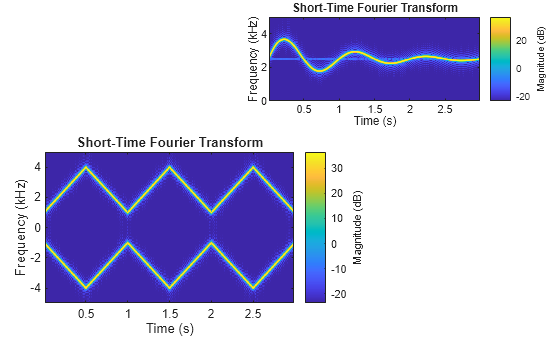
在目标坐标区中绘制 STFT

在新图窗窗口的西南角和东北角创建两个坐标区。

fig = figure;
ax1 = axes(fig,Position=[0.08 0.1 0.55 0.45]);
ax2 = axes(fig,Position=[0.48 0.7 0.48 0.25]);

分别在图窗的西南和东北坐标区中绘制信号 x1 和 x2 的幅值平方 STFT。显示 x2 的 STFT 的单边频率范围。使用包含 256 个采样的凯塞窗、长度为 220 个采样的重叠和 512 个 DFT 点。

g = kaiser(256,5);
ol = 220;
nfft = 512;

stft(x1,Fs,Window=g,OverlapLength=ol,FFTLength=nfft,Parent=ax1)
stft(x2,Fs,Window=g,OverlapLength=ol,FFTLength=nfft, ...
    FrequencyRange="onesided",Parent=ax2)

Figure contains 2 axes objects. Axes object 1 with title Short-Time Fourier Transform, xlabel Time (s), ylabel Frequency (kHz) contains an object of type image. Axes object 2 with title Short-Time Fourier Transform, xlabel Time (s), ylabel Frequency (kHz) contains an object of type image.

在目标 UI 坐标区中绘制 STFT

在新 UI 图窗窗口的西北角创建一个坐标区。

uif = uifigure(Position=[100 100 720 540]);
ax3 = uiaxes(uif,Position=[5 305 300 200]);

在图窗坐标区上绘制信号 x3 的幅值平方 STFT。

stft(x3,Fs,Window=g,OverlapLength=ol,FFTLength=nfft,Parent=ax3)
title(ax3,"STFT in UI Axes")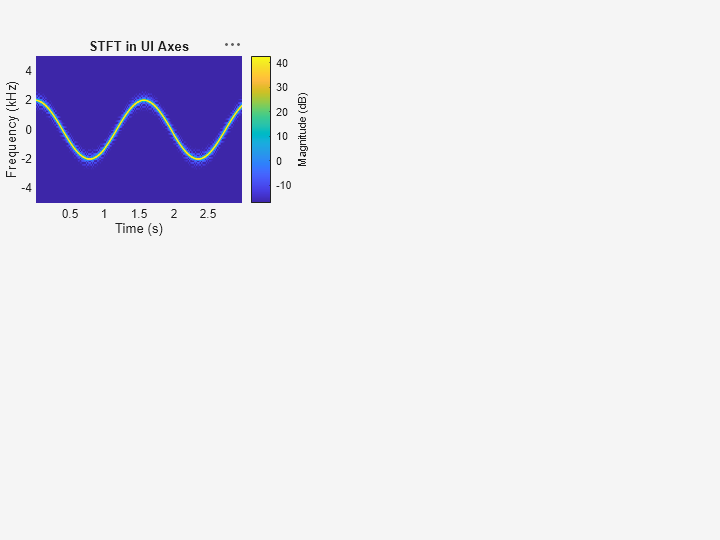

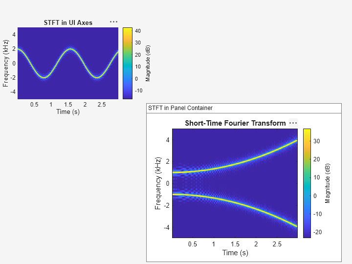
Figure contains an axes object. The axes object with title STFT in UI Axes, xlabel Time (s), ylabel Frequency (kHz) contains an object of type image.

在目标面板容器中绘制 STFT

在 UI 图窗窗口的东南角添加一个面板容器。

p = uipanel(uif,Position=[300 5 400 325], ...
    Title="STFT in Panel Container", ...
    BackgroundColor="white");

在面板容器上绘制信号 x4 的幅值平方 STFT。

stft(x4,Fs,Window=g,OverlapLength=ol,FFTLength=nfft,Parent=p)

Figure contains 2 axes objects and another object of type uipanel. Axes object 1 with title Short-Time Fourier Transform, xlabel Time (s), ylabel Frequency (kHz) contains an object of type image. Axes object 2 with title STFT in UI Axes, xlabel Time (s), ylabel Frequency (kHz) contains an object of type image.

输入参数

`x` — 输入信号
向量 | 矩阵 | 时间表

输入信号，指定为向量、矩阵或 MATLAB^® timetable。

注意

如果您需要 x 和 s 长度相同，则 (length(x)-noverlap)/(length(window)-noverlap) 的值必须为整数。使用 Window 指定 window 的长度，使用 OverlapLength 指定 noverlap。

如果输入有多个通道，请将 x 指定为矩阵，其中每列对应一个通道。
对于时间表输入，x 必须包含均匀递增的有限行时间。如果时间表有缺失或重复的时间点，您可以使用清理包含缺失、重复或不均匀时间的时间表中的提示进行修复。
对于多通道时间表输入，将 x 指定为具有单个变量（其中包含一个矩阵）的时间表，或指定为具有多个变量（其中每个变量包含一个列向量）的时间表。所有变量必须具有相同的精度。

x 的每个通道的长度必须大于或等于窗长度。

示例: chirp(0:1/4e3:2,250,1,500,"quadratic") 指定一个单通道啁啾。

示例: timetable(rand(5,2),SampleRate=1) 指定一个在 1 Hz 下采样 4 秒的双通道随机变量。

示例: timetable(rand(5,1),rand(5,1),SampleRate=1) 指定一个在 1 Hz 下采样 4 秒的双通道随机变量。

数据类型: double | single
复数支持: 是

`fs` — 采样率
`2π` (默认) | 正标量

采样率，指定为正标量。此参量仅当 x 是向量或矩阵时适用。

数据类型: double | single

`ts` — 采样时间
持续时间标量

采样时间，指定为 duration 标量。此参量仅当 x 是向量或矩阵时适用

示例: seconds(1) 是 duration 标量，表示连续信号采样之间有 1 秒时间差。

数据类型: duration

名称-值参数

将可选参量对组指定为 Name1=Value1,...,NameN=ValueN，其中 Name 是参量名称，Value 是对应的值。名称-值参量必须出现在其他参量之后，但对各个参量对组的顺序没有要求。

示例: s = stft(x,Window=hamming(100),OverlapLength=50,FFTLength=128) 使用长度为 100 个采样的汉明窗计算 x 的 STFT，相邻段之间有 50 个采样的重叠且 FFT 包含 128 个点。

`Window` — 频谱窗口
`hann(128,"periodic")` (默认) | 向量

频谱窗，指定为向量。如果您未指定窗或将其指定为空，则函数使用长度为 128 的汉宁窗。Window 的长度必须大于或等于 2。

有关可用窗的列表，请参阅加窗法。

示例: hann(N+1) 和 (1-cos(2*pi*(0:N)'/N))/2 都指定长度为 N + 1 的汉宁窗。

数据类型: double | single

`OverlapLength` — 重叠采样的数量
窗长度的 `75%` (默认) | 非负整数

重叠采样的数量，指定为小于 Window 长度的正整数。如果您省略 OverlapLength 或将其指定为空，则它设置为小于窗长度的 75% 的最大整数，对于默认汉宁窗为 96 个采样。

数据类型: double | single

`FFTLength` — DFT 点数
`128` (默认) | 正整数

DFT 点数，指定为正整数。该值必须大于或等于窗长度。如果输入信号的长度小于 DFT 长度，则数据用零填充。

数据类型: double | single

`FrequencyRange` — STFT 频率范围
`"centered"` (默认) | `"twosided"` | `"onesided"`

STFT 频率范围，指定为 "centered"、"twosided" 或 "onesided"。

"centered" - 计算一个双边、居中 STFT。如果 FFTLength 是偶数，则 s 在区间 (–π, π] 弧度/采样点上计算。如果 FFTLength 是奇数，则 s 在区间 (–π, π) 弧度/采样点上计算。如果您指定时间信息，则区间分别为 (–f_s, f_s/2] 周期/单位时间和 (–f_s, f_s/2) 周期/单位时间，其中 f_s 是有效采样率。
"twosided" - 在区间 [0, 2π) 弧度/采样点上计算双边 STFT。如果您指定时间信息，则区间为 [0, f_s) 周期/单位时间。
"onesided" - 计算单边 STFT。如果 FFTLength 是偶数，则 s 在区间 [0, π] 弧度/采样点上计算。如果 FFTLength 是奇数，则 s 在区间 [0, π) 弧度/采样点上计算。如果您指定时间信息，则区间分别为 [0, f_s/2] 周期/单位时间和 [0, f_s/2) 周期/单位时间，其中 f_s 是有效采样率。此选项仅对实信号有效。
注意
当此参量设置为 "onesided" 时，stft 输出正奈奎斯特范围内的值，并且不保持总功率。

有关示例，请参阅STFT 频率范围。

数据类型: char | string

`OutputTimeDimension` — 输出时间维度
`"acrosscolumns"` (默认) | `"downrows"`

输出时间维度，指定为 "acrosscolumns" 或 "downrows"。如果希望将 s 的时间维度沿行排列，频率维度沿列排列，请将此值设置为 "downrows"。如果希望将 s 的时间维度沿列排列，频率维度沿行排列，请将此值设置为 "acrosscolumns"。如果不带输出参量调用该函数，则忽略此输入。

`Parent` — 目标父容器
`[]` (默认) | `Axes` 对象 | `UIAxes` 对象 | `Panel` 对象

自 R2026a 起

目标父容器，指定为 Axes 对象、UIAxes 对象或 Panel 对象。

如果指定 Parent，则无论是否使用输出参量调用函数，stft 函数都会在指定的目标父容器上将幅值平方 STFT 绘制为曲面图。

有关 MATLAB 图形中目标容器和父子关系的详细信息，请参阅图形对象层次结构。有关在 UIAxes 和 Panel 对象中使用 Parent 设计 App 的详细信息，请参阅Plot Spectral Representations of Signal in App Designer。

输出参量

`s` — 短时傅里叶变换
矩阵 | 三维数组

短时傅里叶变换，以矩阵或三维数组形式返回。时间按 s 的列从左到右递增，频率按行从上到下递增。第三个维度（如果存在）对应一个输入通道。

如果信号 x 有 N_x 个时间采样，则 s 有 k 列，其中 k = ⌊(N_x–L)/(M–L)⌋，M 是 Window 的长度，L 是 OverlapLength，⌊ ⌋ 符号表示向下取整函数。
s 中的行数等于在 FFTLength 中指定的值。

数据类型: double | single

`f` — 频率
向量

在其上计算 STFT 的频率，以向量形式返回。

数据类型: double | single

`t` — 时刻
向量

时刻，以向量形式返回。t 包含时间值，这些时间值对应于用于估计短时功率谱估计值的数据段中心。

如果提供了采样率 fs，则向量包含以秒为单位的时间值。
如果提供了采样时间 ts，则向量是持续时间数组，具有与输入相同的时间格式。
如果未提供时间信息，则向量包含采样编号。

数据类型: double | single

详细信息