Time-Frequency Gallery
This gallery provides you with an overview of the time-frequency analysis features available in Signal Processing Toolbox™ and Wavelet Toolbox™. The descriptions and usage examples present various methods that you can use for your signal analysis.
| Method | Features | Invertible | Examples |
|---|---|---|---|
|
|
| |
| Yes |
| |
| No |
| |
|
|
| |
| Yes |
| |
|
|
|
Short-Time Fourier Transform (Spectrogram)
Description
The short-time Fourier transform is a linear time-frequency representation useful in the analysis of nonstationary multicomponent signals.
The spectrogram is the magnitude squared of the STFT. For more information about computing the spectrogram, see Spectrogram Computation with Signal Processing Toolbox.
The short-time Fourier transform is invertible.
You can compute the cross-spectrogram of two signals to look for similarities in time-frequency space.
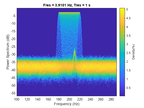
The persistence spectrum of a signal is a time-frequency view that shows the percentage of the time that a given frequency is present in a signal. The persistence spectrum is a histogram in power-frequency space. The longer a particular frequency persists in a signal as the signal evolves, the higher its time percentage and thus the brighter or "hotter" its color in the display.
Potential Applications
The applications of this time-frequency method include, but are not limited to:
Audio signal processing: Fundamental frequency estimation, cross synthesis, spectral envelope extraction, time-scale modification, time-stretching, and pitch shifting. (See Phase Vocoder with Different Synthesis and Analysis Windows for more details.)
Crack detection: Detect cracks in aluminum plates using dispersion curves of ultrasonic Lamb waves.
Sensor array processing: Sonar exploration, geophysical exploration, and beamforming.
Digital communications: Detection of frequency hopping signal.
How to Use
stftcomputes the short-time Fourier transform. To invert the short-time Fourier transform, use theistftfunction.dlstftcomputes the deep learning short-time Fourier transform.dlistftcomputes the deep learning inverse short-time Fourier transform. You must have Deep Learning Toolbox™ installed.stftLayercomputes the short-time Fourier transform within a deep learning network.istftLayercomputes the inverse short-time Fourier transform within a deep learning network. You must have Deep Learning Toolbox installed.stftmag2sigreconstructs a signal starting with the magnitude of its time-frequency representation. You must have Deep Learning Toolbox installed.pspectrumorspectrogramcomputes the spectrogram.xspectrogramcomputes the cross-spectrogram of two signals.signalFrequencyFeatureExtractorextracts frequency-domain features from a signal. You can use the extracted features to train a machine learning model or a deep learning network.signalTimeFeatureExtractorextracts time-domain features from a signal. You can use the extracted features to train a machine learning model or a deep learning network.signalTimeFrequencyFeatureExtractorextracts time-frequency-domain features starting from signal spectrograms, scalograms, wavelet-based decompositions, or data-adaptive methods. You can use the extracted features to train a machine learning model or a deep learning network.You can also use the spectrogram view in Signal Analyzer to view the spectrogram of a signal.
Use the persistence spectrum option in
pspectrumor Signal Analyzer to identify signals hidden in other signals.
Example: Pulses and Oscillations
Generate a signal sampled at 5 kHz for 4 seconds. The signal consists of a set of pulses of decreasing duration separated by regions of oscillating amplitude and fluctuating frequency with an increasing trend.
fs = 5000;
t = 0:1/fs:4-1/fs;

x = 10*besselj(0,1000*(sin(2*pi*(t+2).^3/60).^5));
Compute and plot the short-time Fourier transform of the signal. Window the signal with a 200-sample Kaiser window with shape factor .
stft(x,fs,Window=kaiser(200,30))

Example: Audio Signal with Decreasing Chirps
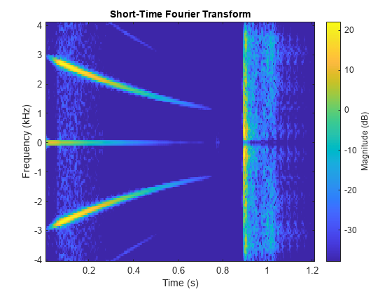
Load an audio signal that contains two decreasing chirps and a wideband splatter sound.
load splatSet the overlap length to 96 samples. Plot the short-time Fourier transform.
stft(y,Fs,OverlapLength=96)
Example: Whale Song
Load a file that contains audio data from a Pacific blue whale, sampled at 4 kHz. The file is from the library of animal vocalizations maintained by the Cornell University Bioacoustics Research Program. The time scale in the data is compressed by a factor of 10 to raise the pitch and make the calls more audible.
[w,fs] = audioread("bluewhale.wav");Compute the spectrogram of the whale song with an overlap percentage equal to eighty percent. Set the minimum threshold for the spectrogram to -50 dB.
pspectrum(w,fs,"spectrogram",Leakage=0.2, ...
    OverlapPercent=80, ...
    MinThreshold=-50)

Example: Persistence Spectrum of Transient Signal
Load an interference narrowband signal embedded within a broadband signal.
load TransientSigCompute the persistence spectrum of the signal. Both signal components are clearly visible.
pspectrum(x,fs,"persistence", ...
    FrequencyLimits=[100 290], ...
    TimeResolution=1)
Continuous Wavelet Transform (Scalogram)
Description
The wavelet transform is a linear time-frequency representation that preserves time shifts and time scalings.
The continuous wavelet transform (CWT) is good at detecting transients in nonstationary signals, and for signals in which instantaneous frequency grows rapidly.
The CWT is invertible.
The CWT tiles the time-frequency plane with variable-size windows. The window automatically widens in time, making it suitable for low-frequency phenomena, and narrows for high frequency phenomena.
Potential Applications
The applications of this time-frequency method include, but are not limited to:
Electrocardiograms (ECG): The most clinically useful information of the ECG signal is found in the time intervals between its consecutive waves and amplitudes defined by its features. The wavelet transform breaks down the ECG signal into scales, making it easier to analyze the ECG signal in different frequency ranges easier to analyze.
Electroencephalogram (EEG): Raw EEG signals suffer from poor spatial resolution, low signal-to-noise ratio, and artifacts. Continuous wavelet decomposition of a noisy signal concentrates intrinsic signal information in a few wavelet coefficients having large absolute values without modifying the random distribution of noise. Therefore, denoising can be achieved by thresholding the wavelet coefficients.
Signal demodulation: Demodulate extended binary phase shift keying (EBPSK) using an adaptive wavelet construction method.
Deep learning: The CWT can be used to create time-frequency representations that can be used to train a convolutional neural network. Classify Time Series Using Wavelet Analysis and Deep Learning (Wavelet Toolbox) shows how to classify ECG signals using scalograms and transfer learning.
How to Use
cwt(Wavelet Toolbox) computes the continuous wavelet transform and displays the scalogram. Alternatively, create a CWT filter bank usingcwtfilterbank(Wavelet Toolbox) and apply thewt(Wavelet Toolbox) function. Use this method to run in parallel applications or when computing the transform for several functions in a loop. To invert the continuous wavelet transform, use theicwt(Wavelet Toolbox) function.dlcwt(Wavelet Toolbox) computes the deep learning CWT. You must have Deep Learning Toolbox installed.cwtLayer(Wavelet Toolbox) computes the CWT within a deep learning network. You must have Deep Learning Toolbox installed.cwtmag2sig(Wavelet Toolbox) reconstructs a signal starting with the scalogram. You must have Deep Learning Toolbox installed.You can use Wavelet Time-Frequency Analyzer (Wavelet Toolbox) to compute and visualize the scalogram of a time series. You can also generate a script to reproduce the CWT analysis in your workspace.
signalTimeFrequencyFeatureExtractorextracts time-frequency-domain features starting from signal spectrograms, scalograms, wavelet-based decompositions, or data-adaptive methods. You can use the extracted features to train a machine learning model or a deep learning network.Signal Analyzer has a scalogram view to visualize the CWT of a time series.
Example: ECG Signal
Load a noisy ECG waveform sampled at 360 Hz.
load ecg
Fs = 360;
Compute the continuous wavelet transform.
cwt(ecg,Fs)

The ECG data is taken from the MIT-BIH Arrhythmia Database [2].
Example: Signal with Transient Events
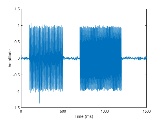
Generate a signal sampled at 1 kHz for 1.5 seconds. The signal consists of two sinusoidal components that turn on and off abruptly, with additional "defects" at 222 milliseconds and 800 milliseconds.
Fs = 1e3;
t = 0:1/Fs:1.5-1/Fs;
addNoise = 0.025*randn(size(t));
x = cos(2*pi*150*t).*(t>=0.1 & t<0.5) + ...
    sin(2*pi*200*t).*(t>0.7 & t<=1.2);
x = x+addNoise;
x([222 800]) = x([222 800])+[-2 2];
plot(t.*1000,x)
xlabel("Time (ms)")
ylabel("Amplitude")
Obtain the CWT of the signal. Use the analytic Morlet wavelet. Plot only the finest-scale wavelet coefficients. Create a second axis and plot the original time data.
cfs = cwt(x,Fs,"amor");
plot(t,abs(cfs(1,:)),LineWidth=2)
ylabel("Magnitude")
set(gca,XTick=[0.1 0.222 0.5 0.7 0.8 1.2])
yyaxis right
plot(t,x,"--")
ylabel("Amplitude")
xlabel("Time(s)")

Wigner-Ville Distribution
Description
The Wigner-Ville distribution (WVD) is a quadratic energy density computed by correlating the signal with a time and frequency translated and complex-conjugated version of itself.
The Wigner-Ville distribution is always real even if the signal is complex.
Time and frequency marginal densities correspond to instantaneous power and spectral energy density, respectively.
The instantaneous frequency and group delay can be evaluated using local first-order moments of the Wigner distribution.
The time resolution of the WVD is equal to the number of input samples.
The Wigner distribution can locally assume negative values.
Potential Applications
The applications of this time-frequency method include, but are not limited to:
Otoacoustic emissions (OAEs): OAEs are narrowband oscillatory signals emitted by the cochlea (inner ear), and their presence is indicative of normal hearing.
Quantum mechanics: Quantum corrections to classical statistical mechanics, model electron transport, and calculate static and dynamic properties of many-body quantum systems.
How to Use
wvdcomputes the Wigner-Ville distribution.xwvdcomputes the cross Wigner-Ville distribution of two signals. See Use Cross Wigner-Ville Distribution to Estimate Instantaneous Frequency for more details.
Example: Otoacoustic Emission
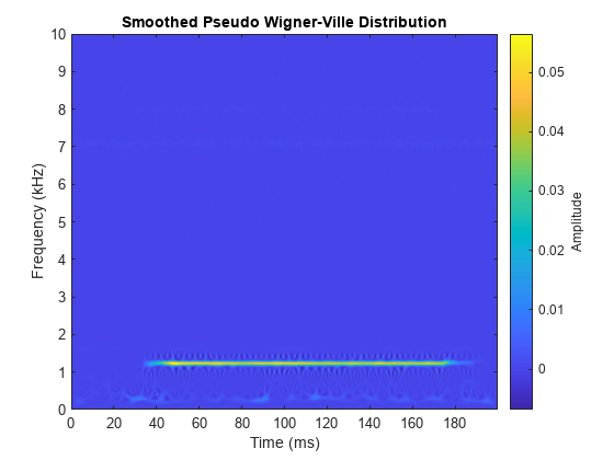
Load a data file containing otoacoustic emission data sampled at 20 kHz. The emission is produced by a stimulus beginning at 25 milliseconds and ending at 175 milliseconds.
load dpoae
Fs = 20e3;
Compute the smoothed-pseudo Wigner Ville distribution of the otoacoustic data. The convenience plot isolates the emission frequency at roughly the expected value 1.2 kHz.
wvd(dpoaets,Fs,"smoothedPseudo",kaiser(511,10),kaiser(511,10), ...
    NumFrequencyPoints=4000, ...
    NumTimePoints=3990)
For more details on otoacoustic emissions, see "Determining Exact Frequency Through the Analytic CWT" in CWT-Based Time-Frequency Analysis (Wavelet Toolbox).
Reassignment and Synchrosqueezing
Description
Reassignment sharpens the localization of spectral estimates and produces spectrograms that are easier to read and interpret. The technique relocates each spectral estimate to the center of energy of its bin instead of the bin's geometric center. It provides exact localization for chirps and impulses.
The Fourier synchrosqueezed transform starts from the short-time Fourier transform and "squeezes" its values so that they concentrate around curves of instantaneous frequency in the time-frequency plane.
The wavelet synchrosqueezed transform reassigns the signal energy in frequency.
Both the Fourier synchrosqueezed transform and the wavelet synchrosqueezed transform are invertible.
The reassigned and synchrosqueezing methods are especially suited to track and extract time-frequency ridges.
Potential Applications
The applications of this time-frequency method include, but are not limited to:
Audio signal processing: Synchrosqueezing transform (SST) was originally introduced in the context of audio signal analysis.
Seismic data: Analysis of seismic data to find oil and gas traps. Synchrosqueezing can also detect deep-layer weak signals that are usually smeared in seismic data.
Oscillations in power systems: A steam turbine and electric generator can have mechanical subsynchronous oscillation (SSO) modes between the various turbine stages and the generator. The frequency of the SSO is generally between 5 Hz and 45 Hz, and the mode frequencies are often close to each other. The antinoise ability and time-frequency resolution of WSST improves the readability of the time-frequency view.
Deep learning: Synchrosqueezed transforms can be used to extract time-frequency features and fed into a network that classifies time-series data. Waveform Segmentation Using Deep Learning shows how
fsstoutputs can be fed into an LSTM network that classifies ECG signals.
How to Use
Use the
'reassigned'option inspectrogram, set the'Reassigned'argument totrueinpspectrum, or check the Reassign box in the spectrogram view of Signal Analyzer to compute reassigned spectrograms.fsstcomputes the Fourier synchrosqueezed transform. Use theifsstfunction to invert the Fourier synchrosqueezed transform. (See Fourier Synchrosqueezed Transform of Speech Signal for reconstruction of speech signals usingifsst.)wsst(Wavelet Toolbox) computes the wavelet synchrosqueezed transform. Use theiwsst(Wavelet Toolbox) function to invert the wavelet synchrosqueezed transform. (See Inverse Synchrosqueezed Transform of Chirp (Wavelet Toolbox) for reconstruction of a quadratic chirp usingiwsst(Wavelet Toolbox).)signalTimeFrequencyFeatureExtractorextracts time-frequency-domain features starting from signal spectrograms, scalograms, wavelet-based decompositions, or data-adaptive methods. You can use the extracted features to train a machine learning model or a deep learning network.
Example: Echolocation Pulse
Load an echolocation pulse emitted by a big brown bat (Eptesicus Fuscus). The sampling interval is 7 microseconds.
load batsignal
Fs = 1/DT;
Compute the reassigned spectrogram of the signal.
tiledlayout(2,1)
nexttile
pspectrum(batsignal,Fs,"spectrogram", ...
    TimeResolution=280e-6, ...
    OverlapPercent=85, ...
    MinThreshold=-45, ...
    Leakage=0.9)
nexttile
pspectrum(batsignal,Fs,"spectrogram", ...
    TimeResolution=280e-6, ...
    OverlapPercent=85, ...
    MinThreshold=-45, ...
    Leakage=0.9, ...
    Reassign=true)
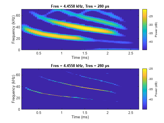
Thanks to Curtis Condon, Ken White, and Al Feng of the Beckman Center at the University of Illinois for the bat data and permission to use it in this example [3].
Example: Speech Signals
Load a file containing the word "strong," spoken by a woman and by a man. The signals are sampled at 8 kHz. Concatenate them into a single signal.
load Strong
x = [her' him'];
Compute the synchrosqueezed Fourier transform of the signal. Window the signal using a Kaiser window with shape factor .
fsst(x,Fs,kaiser(256,20),"yaxis")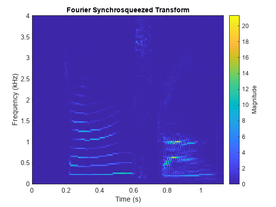
Example: Synthetic Seismic Data
Load the synthetic seismic data sampled at 100 Hz for 1 second.
load SyntheticSeismicDataThe workspace now contains the synthetic data, x, and a sample rate, Fs.
Compute the wavelet synchrosqueezed transform of the seismic data using the bump wavelet and 30 voices per octave. Specify zero padding as the boundary extension mode.
wsst(x,Fs,"bump", ...
    VoicesPerOctave=30, ...
    Boundary="zeropad")

The seismic signal is generated using the two sinusoids mentioned in "Time-Frequency Analysis of Seismic Data Using Synchrosqueezing Transform" by Ping Wang, Jinghuai Gao, and Zhiguo Wang [4].
Example: Earthquake Vibration
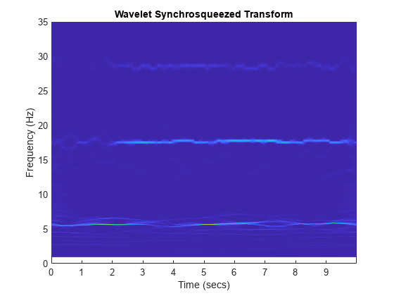
Load acceleration measurements recorded on the first floor of a three story test structure under earthquake conditions. The measurements are sampled at 1 kHz.
load quakevib
Fs = 1e3;
Compute the wavelet synchrosqueezed transform of the acceleration measurements. You are analyzing vibration data that exhibit a cyclic behavior. The synchrosqueezed transform allows you to isolate the three frequency components, separated by roughly 11 Hz. The main vibration frequency is at 5.86 Hz, and the equispaced frequency peaks suggest that they are harmonically related. The cyclic behavior of the vibrations is also visible.
wsst(gfloor1OL,Fs,"bump", ...
    VoicesPerOctave=48)
ylim([0 35])
Example: Kobe Earthquake Data
Load seismograph data recorded during the 1995 Kobe earthquake. The data has a sample rate of 1 Hz.
load kobe
Fs = 1;
Compute the wavelet synchrosqueezed transform that isolates the different frequency components of the seismic data.
wsst(kobe,Fs,"bump", ...
    VoicesPerOctave=48)
ylim([0 300])
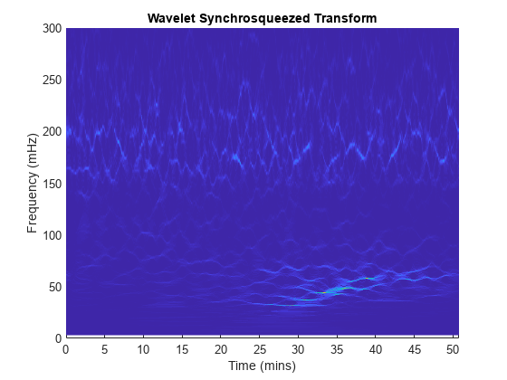
The data are seismograph (vertical acceleration, nm/sq.sec) measurements recorded at Tasmania University, Hobart, Australia on 16 January 1995 beginning at 20:56:51 (GMT) and continuing for 51 minutes at 1 second intervals [5].
Example: Subsynchronous Oscillation in Power Systems
Load the subsynchronous oscillation data of a Power System.
load OscillationDataCompute the wavelet synchrosqueezed transform using the bump wavelet and 48 voices per octave. The four mode frequencies are at 15 Hz, 20 Hz, 25 Hz and 32 Hz. Notice that the energies of the modes at 15 Hz and 20 Hz decrease with time, whereas the energy of the modes at 25 Hz and 32 Hz increase gradually over time.
wsst(x,Fs,"bump", ...
    VoicesPerOctave=48)
ylim([10 50])
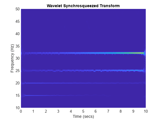
This synthetic subsynchronous oscillation data was generated using the equation defined by Zhao et al in "Application of Synchrosqueezed Wavelet Transforms for Extraction of the Oscillatory Parameters of Subsynchronous Oscillation in Power Systems" [6].
Constant-Q Gabor Transform
Description
The constant-Q nonstationary Gabor transform uses windows with different center frequencies and bandwidths such that the ratio of center frequency to bandwidth, the Q factor, remains constant.
The constant-Q Gabor transform enables the construction of stable inverses, yielding perfect signal reconstruction.
In frequency space, the windows are centered at logarithmically spaced frequencies up to the Nyquist frequency. The smallest allowable center frequency is Fs/N, where Fs is the sample rate and N is the number of samples.
Potential Applications
The applications of this time-frequency method include, but are not limited to:
Audio signal processing: The fundamental frequencies of the tones in music are geometrically spaced. The frequency resolution of the human auditory system is approximately constant-Q, making this technique appropriate for music signal processing.
How to Use
Example: Rock Music
Load an audio file containing a fragment of rock music with vocals, drums, and guitar. The signal has a sample rate of 44.1 kHz.
load drumsSet the frequency range from the smallest allowable center frequency to 2 kHz. Compute the CQT of the signal using 20 bins per octave.
minFreq = fs/length(audio);
maxFreq = 2e3;
cqt(audio, ...
    SamplingFrequency=fs, ...
    BinsPerOctave=20, ...
    FrequencyLimits=[minFreq maxFreq])

Data-Adaptive Methods and Multiresolution Analysis
Description
The empirical mode decomposition decomposes the signals into intrinsic mode functions which form a complete and nearly orthogonal basis for the original signal.
The variational mode decomposition decomposes a signal into a small number of narrowband intrinsic mode functions. The method simultaneously calculates all the mode waveforms and their central frequencies by optimizing a constrained variational problem.
The empirical wavelet transform decomposes the signals into multiresolution analysis (MRA) components. The method uses an adaptable wavelet subdivision scheme that automatically determines the empirical wavelet and scaling filters and preserves energy.
The Hilbert-Huang transform computes the instantaneous frequency of each intrinsic mode function.
The maximal overlap discrete wavelet transform (MODWT) partitions a signal's energy across detail and scaling coefficients. The MODWT is a nondecimated discrete wavelet transform useful for applications that require a shift-invariant transform. You can obtain multiscale variance and correlation estimates, and invert the transform.
The tunable Q-factor wavelet transform provides a Parseval frame decomposition where energy is partitioned among components, as well as perfect reconstruction of the signal. The tunable Q-factor wavelet transform is a technique that creates an MRA with a user-specified Q-factor. The Q-factor is the ratio of the center frequency to the bandwidth of the filters used in the transform.
These methods combined are useful for analyzing nonlinear and nonstationary signals.
Potential Applications
The applications of this time-frequency method include, but are not limited to:
Physiological signal processing: Analyze human EEG response to transcranial magnetic stimulation (TMS) of the brain cortex.
Structural applications: Locate anomalies that appear as cracks, delamination, or stiffness loss in beams and plates.
System identification: Isolate modal damping ratios of structures with closely spaced modal frequencies.
Ocean engineering: Identify transient electromagnetic disturbances caused by humans in underwater electromagnetic environments.
Solar physics: Extract periodic components of sunspot data.
Atmospheric turbulence: Observe stable boundary layer to separate turbulent and nonturbulent motions.
Epidemiology: Assess traveling speed of communicative diseases such as Dengue fever.
How to Use
emdcomputes the empirical mode decomposition.vmdcomputes the variational mode decomposition.ewt(Wavelet Toolbox) computes the empirical wavelet transform.hhtcomputes the Hilbert Huang spectrum of an empirical mode decomposition.modwpt(Wavelet Toolbox) computes the maximal overlap discrete wavelet packet transform. To invert the MODWPT transform, use theimodwpt(Wavelet Toolbox) function. To obtain the MODWPT details, usemodwptdetails(Wavelet Toolbox). The MODWPT details provide zero-phase filtering of the signal.modwt(Wavelet Toolbox) computes the maximal overlap discrete wavelet transform. To invert the MODWT, use theimodwt(Wavelet Toolbox) function. To obtain the MRA analysis, usemodwtmra(Wavelet Toolbox).modwtLayer(Wavelet Toolbox) computes the computes the MODWT and MODWT multiresolution analysis (MRA) of the input. You must have Deep Learning Toolbox installed.tqwt(Wavelet Toolbox) computes the tunable Q-factor wavelet transform. To invert the TQWT, use theitqwt(Wavelet Toolbox) function. To obtain the MRA analysis, usetqwtmra(Wavelet Toolbox).signalTimeFrequencyFeatureExtractorextracts time-frequency-domain features starting from signal spectrograms, scalograms, wavelet-based decompositions, or data-adaptive methods. You can use the extracted features to train a machine learning model or a deep learning network.You can use Signal Multiresolution Analyzer (Wavelet Toolbox) to visualize multilevel wavelet- and data adaptive-based decompositions of real-valued 1-D signals.
Wavelet Signal Analyzer (Wavelet Toolbox) enables visualization, analysis, and compression of 1-D signals using decimated and nondecimated discrete wavelet and wavelet packet transforms.
Example: Bearing Vibration
Load the vibration signal from a defective bearing generated in the Compute Hilbert Spectrum of Vibration Signal example. The signal is sampled at a rate 10 kHz.
load bearingVibrationCompute the first five intrinsic mode functions (IMFs) of the signal. Plot the Hilbert spectrum of the first and third empirical modes. The first mode reveals increasing wear due to high-frequency impacts on the bearing's outer race. The third mode shows a resonance occurring halfway through the measurement process that caused the defect in the bearing.
imf = emd(y, ...
    MaxNumIMF=5, ...
    Display=0);
tiledlayout(2,1)
nexttile
hht(imf(:,1),fs)
nexttile
hht(imf(:,3),fs, ...
    FrequencyLimits=[0 100])

References
[1] The Pacific blue whale file is obtained from the library of animal vocalizations maintained by the Cornell University Bioacoustics Research Program.
[2] Moody G. B, Mark R. G. The impact of the MIT-BIH Arrhythmia Database. IEEE Eng in Med and Biol 20(3):45-50 (May-June 2001). (PMID: 11446209)
[3] Thanks to Curtis Condon, Ken White, and Al Feng of the Beckman Center at the University of Illinois for the bat echolocation data.
[4] Wang, Ping, Gao, J., and Wang, Z. Time-Frequency Analysis of Seismic Data Using Synchrosqueezing Transform, IEEE Geoscience and Remote Sensing Letters, Vol 12, Issue 11, Dec. 2014.
[5] Seismograph (vertical acceleration, nm/sq.sec) of the Kobe earthquake, recorded at Tasmania University, Hobart, Australia on 16 January 1995 beginning at 20:56:51 (GMTRUE) and continuing for 51 minutes at 1 second intervals.
[6] Zhao et al. Application of Synchrosqueezed Wavelet Transforms for Extraction of the Oscillatory Parameters of Subsynchronous Oscillation in Power Systems MDPI Energies; Published 12 June 2018.
[7] Boashash, Boualem. Time-Frequency Signal Analysis and Processing: A Comprehensive Reference Elsevier, 2016.
See Also
Apps
- Signal Analyzer | Signal Multiresolution Analyzer (Wavelet Toolbox) | Wavelet Signal Analyzer (Wavelet Toolbox) | Wavelet Time-Frequency Analyzer (Wavelet Toolbox)
Objects
cwtLayer(Wavelet Toolbox) |modwtLayer(Wavelet Toolbox) |istftLayer|signalFrequencyFeatureExtractor|signalTimeFeatureExtractor|signalTimeFrequencyFeatureExtractor|stftLayer
Functions
cqt(Wavelet Toolbox) |cwt(Wavelet Toolbox) |cwtfilterbank(Wavelet Toolbox) |cwtmag2sig(Wavelet Toolbox) |dlcwt(Wavelet Toolbox) |dlistft|dlstft|emd|ewt(Wavelet Toolbox) |fsst|hht|icqt(Wavelet Toolbox) |icwt(Wavelet Toolbox) |ifsst|imodwpt(Wavelet Toolbox) |imodwt(Wavelet Toolbox) |istft|itqwt(Wavelet Toolbox) |iwsst(Wavelet Toolbox) |kurtogram|modwpt(Wavelet Toolbox) |modwptdetails(Wavelet Toolbox) |modwt(Wavelet Toolbox) |modwtmra(Wavelet Toolbox) |pspectrum|spectralKurtosis|spectrogram|stft|stftmag2sig|tqwt(Wavelet Toolbox) |tqwtmra(Wavelet Toolbox) |vmd|wsst(Wavelet Toolbox) |wt(Wavelet Toolbox) |xspectrogram|wvd|xwvd