Extract Features of a Clock Signal
How sharply does an on/off signal turn on and off? How often and for how long is it activated? Determine all those characteristics for the output of a clock.
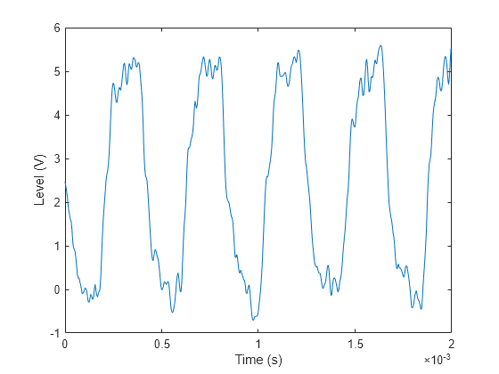
Load the signal and plot it. The time is measured in seconds and the level in volts.
load('clock.mat')

plot(tclock,clocksig)
xlabel('Time (s)')
ylabel('Level (V)')
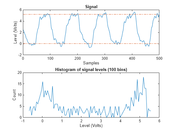
Use statelevels to find the lower and upper levels of the signal by means of a histogram. If you do not specify an output, the function plots the signal, marks the levels, and displays the histogram.
levels = statelevels(clocksig)
levels = 1×2

    0.0138    5.1848
statelevels(clocksig);
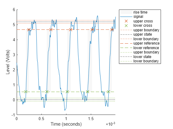
Determine how fast the signal rises at each transition. risetime uses the lower and upper levels found by statelevels. It defines the rise time as the time it takes the signal to rise from 10% to 90% of the difference between the levels.
[Rise,LoTime,HiTime,LoLev,HiLev] = risetime(clocksig,tclock);

Levels = [LoLev HiLev; (levels(2)-levels(1))*[0.1 0.9]+levels(1)]
Levels = 2×2

    0.5309    4.6677
    0.5309    4.6677
If you call risetime without outputs, the function draws an annotated plot of the signal. The rise times are shaded, the crossing points are marked, and the levels are displayed. You can use the time vector or the sample rate as input.
risetime(clocksig,Fs);
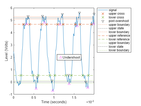
overshoot and undershoot show how far the signal deviates from the state levels at each transition. The results are expressed as percentages of the difference between the levels. Further outputs give the actual times and signal values.
overshoot(clocksig,Fs);

[pctgs,values,times] = undershoot(clocksig,Fs);

hold on
text(1.1e-3,2,'     Undershoot','Background','w','Edge','k')
plot([times;1.17e-3],[values;2],'^m','HandleVisibility','off')
hold off
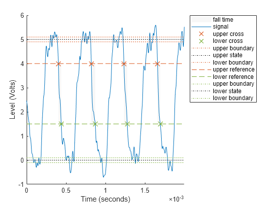
Determine how fast the signal falls using falltime. You can set the state levels and the percentage reference levels manually. You can do the same with risetime.
falltime(clocksig,tclock, ...
    'PercentReferenceLevels',[30 80],'StateLevels',[0 5]);
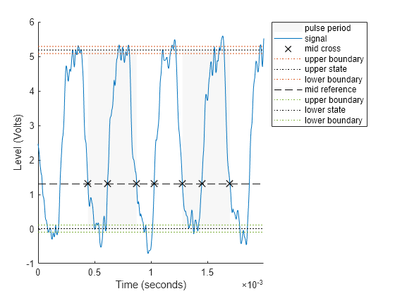
Find the period of the signal. By default, the period is defined as the time elapsed between consecutive rising crossings of the reference level halfway between the state levels. You can change the polarity of the crossings, specify the state levels, or adjust the reference level.
per = pulseperiod(clocksig,tclock)
per = 4×1
10-3 ×

    0.4143
    0.4200
    0.4188
    0.4111
pulseperiod(clocksig,Fs,'Polarity','negative','MidPct',25);
The duty cycle is the ratio of pulse width to pulse period. Determine it directly or using a dedicated function.
dut = dutycycle(clocksig,Fs);

wdt = pulsewidth(clocksig,Fs);

compare = [wdt./per dut]
compare = 4×2

    0.4862    0.4862
    0.4756    0.4756
    0.4871    0.4871
    0.4886    0.4886
See Also
dutycycle | falltime | overshoot | pulseperiod | pulsewidth | risetime | slewrate | statelevels | undershoot