Interpret Machine Learning Models

This topic introduces Statistics and Machine Learning Toolbox™ features for model interpretation and shows how to interpret a machine learning model (classification and regression).

A machine learning model is often referred to as a "black box" model because it can be difficult to understand how the model makes predictions. Interpretability tools help you overcome this aspect of machine learning algorithms and reveal how predictors contribute (or do not contribute) to predictions. Also, you can validate whether the model uses the correct evidence for its predictions, and find model biases that are not immediately apparent.

Features for Model Interpretation

Use lime, shapley, and plotPartialDependence to explain the contribution of individual predictors to the predictions of a trained classification or regression model.

lime — Local interpretable model-agnostic explanations (LIME [1]) interpret a prediction for a query point by fitting a simple interpretable model for the query point. The simple model acts as an approximation for the trained model and explains model predictions around the query point. The simple model can be either a linear model or a decision tree model. You can use the estimated coefficients of a linear model or the estimated predictor importance of a decision tree model to explain the contribution of individual predictors to the prediction for the query point. For more details, see LIME.
shapley — The Shapley value ([2], [3], and [4]) of a predictor for a query point explains the deviation of the prediction (response for regression or class scores for classification) for the query point from the average prediction, due to the predictor. For a query point, the sum of the Shapley values for all features corresponds to the total deviation of the prediction from the average. For more details, see Shapley Values for Machine Learning Model.
plotPartialDependence and partialDependence — A partial dependence plot (PDP [5]) shows the relationships between a predictor (or a pair of predictors) and the prediction (response for regression or class scores for classification) in the trained model. The partial dependence on the selected predictor is defined by the averaged prediction obtained by marginalizing out the effect of the other variables. Therefore, the partial dependence is a function of the selected predictor that shows the average effect of the selected predictor over the data set. You can also create a set of individual conditional expectation (ICE [6]) plots for each observation, showing the effect of the selected predictor on a single observation. For more details, see More About on the plotPartialDependence reference page.

Some machine learning models support embedded type feature selection, where the model learns predictor importance as part of the model learning process. You can use the estimated predictor importance to explain model predictions. For example:

Train an ensemble (ClassificationBaggedEnsemble or RegressionBaggedEnsemble) of bagged decision trees (for example, random forest) and use the predictorImportance and oobPermutedPredictorImportance functions.
Train a linear model with lasso regularization, which shrinks the coefficients of the least important predictors. Then use the estimated coefficients as measures for predictor importance. For example, use fitclinear or fitrlinear and specify the 'Regularization' name-value argument as 'lasso'.

For a list of machine learning models that support embedded type feature selection, see Embedded Type Feature Selection.

Use Statistics and Machine Learning Toolbox features for three levels of model interpretation: local, cohort, and global.

Level	Objective	Use Case	Statistics and Machine Learning Toolbox Feature
Local interpretation	Explain a prediction for a single query point.	Identify important predictors for an individual prediction. Examine a counterintuitive prediction.	Use `lime` and `shapley` for a specified query point.
Cohort interpretation	Explain how a trained model makes predictions for a subset of the entire data set.	Validate predictions for a particular group of samples.	Use `lime` and `shapley` for multiple query points. After creating a `lime` or `shapley` object, you can call the object function `fit` multiple times to interpret predictions for other query points. Pass a subset of data when you call `lime`, `shapley`, and `plotPartialDependence`. The features interpret the trained model using the specified subset instead of the entire training data set.
Global interpretation	Explain how a trained model makes predictions for the entire data set.	Demonstrate how a trained model works. Compare different models.	Use `plotPartialDependence` to create PDPs and ICE plots for the predictors of interest. Use `shapley` to compute Shapley values for all observations. Visualize the results by using the `plot`, `boxchart`, `plotDependence`, or `swarmchart` object functions. Find important predictors from a trained model that supports Embedded Type Feature Selection.

Interpret Classification Model

Open Live Script

This example trains an ensemble of bagged decision trees using the random forest algorithm, and interprets the trained model using interpretability features. Use the object functions (oobPermutedPredictorImportance and predictorImportance) of the trained model to find important predictors in the model. Also, use lime and shapley to interpret the predictions for specified query points. Then use plotPartialDependence to create a plot that shows the relationships between an important predictor and predicted classification scores.

Train Classification Ensemble Model

Load the CreditRating_Historical data set. The data set contains customer IDs and their financial ratios, industry labels, and credit ratings.

tbl = readtable('CreditRating_Historical.dat');

Display the first three rows of the table.

head(tbl,3)

     ID      WC_TA    RE_TA    EBIT_TA    MVE_BVTD    S_TA     Industry    Rating
    _____    _____    _____    _______    ________    _____    ________    ______

    62394    0.013    0.104     0.036      0.447      0.142       3        {'BB'}
    48608    0.232    0.335     0.062      1.969      0.281       8        {'A' }
    42444    0.311    0.367     0.074      1.935      0.366       1        {'A' }

Create a table of predictor variables by removing the columns containing customer IDs and ratings from tbl.

tblX = removevars(tbl,["ID","Rating"]);

Train an ensemble of bagged decision trees by using the fitcensemble function and specifying the ensemble aggregation method as random forest ('Bag'). For reproducibility of the random forest algorithm, specify the 'Reproducible' name-value argument as true for tree learners. Also, specify the class names to set the order of the classes in the trained model.

rng('default') % For reproducibility
t = templateTree('Reproducible',true);
blackbox = fitcensemble(tblX,tbl.Rating, ...
    'Method','Bag','Learners',t, ...
    'CategoricalPredictors','Industry', ...
    'ClassNames',{'AAA' 'AA' 'A' 'BBB' 'BB' 'B' 'CCC'});

blackbox is a ClassificationBaggedEnsemble model.

Use Model-Specific Interpretability Features

ClassificationBaggedEnsemble supports two object functions, oobPermutedPredictorImportance and predictorImportance, which find important predictors in the trained model.

Estimate out-of-bag predictor importance by using the oobPermutedPredictorImportance function. The function randomly permutes out-of-bag data across one predictor at a time, and estimates the increase in the out-of-bag error due to this permutation. The larger the increase, the more important the feature.

Imp1 = oobPermutedPredictorImportance(blackbox);

Estimate predictor importance by using the predictorImportance function. The function estimates predictor importance by summing changes in the node risk due to splits on each predictor and dividing the sum by the number of branch nodes.

Imp2 = predictorImportance(blackbox);

Create a table containing the predictor importance estimates, and use the table to create horizontal bar graphs. To display an existing underscore in any predictor name, change the TickLabelInterpreter value of the axes to 'none'.

table_Imp = table(Imp1',Imp2', ...
    'VariableNames',{'Out-of-Bag Permuted Predictor Importance','Predictor Importance'}, ...
    'RowNames',blackbox.PredictorNames);
tiledlayout(1,2)
ax1 = nexttile;
table_Imp1 = sortrows(table_Imp,'Out-of-Bag Permuted Predictor Importance');
barh(categorical(table_Imp1.Row,table_Imp1.Row),table_Imp1.('Out-of-Bag Permuted Predictor Importance'))
xlabel('Out-of-Bag Permuted Predictor Importance')
ylabel('Predictor')
ax2 = nexttile;
table_Imp2 = sortrows(table_Imp,'Predictor Importance');
barh(categorical(table_Imp2.Row,table_Imp2.Row),table_Imp2.('Predictor Importance'))
xlabel('Predictor Importance')
ax1.TickLabelInterpreter = 'none';
ax2.TickLabelInterpreter = 'none';

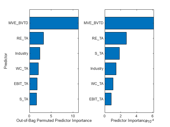
Figure contains 2 axes objects. Axes object 1 with xlabel Out-of-Bag Permuted Predictor Importance, ylabel Predictor contains an object of type bar. Axes object 2 with xlabel Predictor Importance contains an object of type bar.

Both object functions identify MVE_BVTD and RE_TA as the two most important predictors.

Specify Query Point

Find the observations whose Rating is 'AAA' and choose four query points among them.

rng('default')
tblX_AAA = tblX(strcmp(tbl.Rating,'AAA'),:);
queryPoint = datasample(tblX_AAA,4,'Replace',false)

queryPoint=4×6 table
    WC_TA    RE_TA    EBIT_TA    MVE_BVTD    S_TA     Industry
    _____    _____    _______    ________    _____    ________

    0.283    0.715     0.069      9.612      1.066       11   
    0.603    0.891     0.117      7.851      0.591        6   
    0.212    0.486     0.057      3.986      0.679        2   
    0.273    0.491     0.071      3.287      0.465        5

Use LIME with Linear Simple Models

Explain the predictions for the query points using lime with linear simple models. lime generates a synthetic data set and fits a simple model to the synthetic data set.

Create a lime object using tblX_AAA so that lime generates a synthetic data set using only the observations whose Rating is 'AAA', not the entire data set.

explainer_lime = lime(blackbox,tblX_AAA);

The default value of DataLocality for lime is 'global', which implies that, by default, lime generates a global synthetic data set and uses it for any query points. lime uses different observation weights so that weight values are more focused on the observations near the query point. Therefore, you can interpret each simple model as an approximation of the trained model for a specific query point.

Fit simple models for the four query points by using the object function fit. Specify the third input (the number of important predictors to use in the simple model) as 6 to use all six predictors.

explainer_lime1 = fit(explainer_lime,queryPoint(1,:),6);
explainer_lime2 = fit(explainer_lime,queryPoint(2,:),6);
explainer_lime3 = fit(explainer_lime,queryPoint(3,:),6);
explainer_lime4 = fit(explainer_lime,queryPoint(4,:),6);

Plot the coefficients of the simple models by using the object function plot.

tiledlayout(2,2)
nexttile
plot(explainer_lime1)
nexttile
plot(explainer_lime2)
nexttile
plot(explainer_lime3)
nexttile
plot(explainer_lime4)

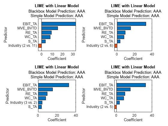
All simple models identify EBIT_TA, MVE_BVTD, RE_TA, and WC_TA as the four most important predictors. The positive coefficients for the predictors suggest that increasing the predictor values leads to an increase in the predicted scores in the simple models.

For a categorical predictor, the plot function displays only the most important dummy variable of the categorical predictor. Therefore, each bar graph displays a different dummy variable.

Compute Shapley Values

The Shapley value of a predictor for a query point explains the deviation of the predicted score for the query point from the average score, due to the predictor. Create a shapley object using tblX_AAA so that shapley computes the expected contribution based on the samples for 'AAA'.

explainer_shapley = shapley(blackbox,tblX_AAA);

Compute the Shapley values for the query points by using the object function fit.

explainer_shapley1 = fit(explainer_shapley,queryPoint(1,:));
explainer_shapley2 = fit(explainer_shapley,queryPoint(2,:));
explainer_shapley3 = fit(explainer_shapley,queryPoint(3,:));
explainer_shapley4 = fit(explainer_shapley,queryPoint(4,:));

Plot the Shapley values by using the object function plot.

tiledlayout(2,2)
nexttile
plot(explainer_shapley1)
nexttile
plot(explainer_shapley2)
nexttile
plot(explainer_shapley3)
nexttile
plot(explainer_shapley4)

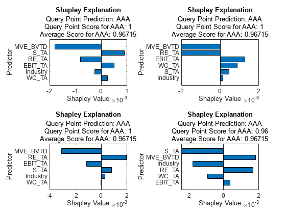
MVE_BVTD is the most important predictor for all the query points. The Shapley values of MVE_BVTD are positive for the first three query points. The MVE_BVTD variable values are about 9.6, 7.9, 4.0, and 3.3 for the query points. According to the Shapley values for the four query points, a large MVE_BVTD value leads to an increase in the predicted score, and a small MVE_BVTD value leads to a decrease in the predicted scores compared to the average.

Create Partial Dependence Plot (PDP)

A PDP plot shows the averaged relationships between the predictor and the predicted score in the trained model. Create PDPs for RE_TA and MVE_BVTD, which the other interpretability tools identify as important predictors. Pass tblx_AAA to plotPartialDependence so that the function computes the expectation of the predicted scores using only the samples for 'AAA'.

figure
plotPartialDependence(blackbox,'RE_TA','AAA',tblX_AAA)

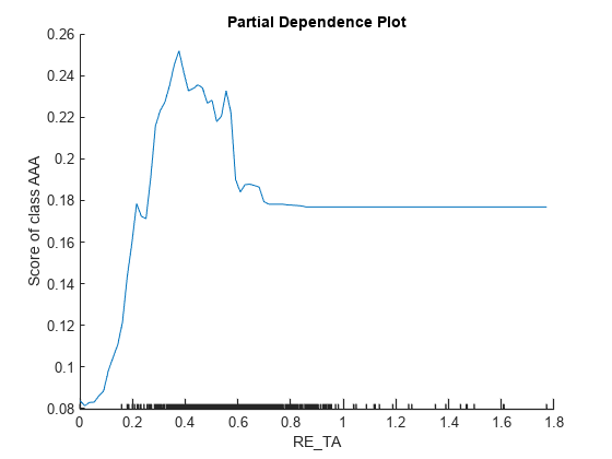
Figure contains an axes object. The axes object with title Partial Dependence Plot, xlabel R E indexOf T baseline A RE_TA, ylabel Score of class AAA contains an object of type line.

plotPartialDependence(blackbox,'MVE_BVTD','AAA',tblX_AAA)

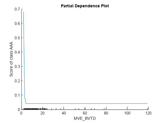
Figure contains an axes object. The axes object with title Partial Dependence Plot, xlabel M V E indexOf B baseline V T D MVE_BVTD, ylabel Score of class AAA contains an object of type line.

The minor ticks in the x-axis represent the unique values of the predictor in tbl_AAA. The plot for MVE_BVTD shows that the predicted score is large when the MVE_BVTD value is small. The score value decreases as the MVE_BVTD value increases until it reaches about 5, and then the score value stays unchanged as the MVE_BVTD value increases. The dependency on MVE_BVTD in the subset tbl_AAA identified by plotPartialDependence is not consistent with the local contributions of MVE_BVTD at the four query points identified by lime and shapley.

Interpret Regression Model

Open Live Script

The model interpretation workflow for a regression problem is similar to the workflow for a classification problem, as demonstrated in the example Interpret Classification Model.

This example trains a Gaussian process regression (GPR) model and interprets the trained model using interpretability features. Use a kernel parameter of the GPR model to estimate predictor weights. Also, use lime and shapley to interpret the predictions for specified query points. Then use plotPartialDependence to create a plot that shows the relationships between an important predictor and predicted responses.

Train GPR Model

Load the carbig data set, which contains measurements of cars made in the 1970s and early 1980s.

load carbig

Create a table containing the predictor variables Acceleration, Cylinders, and so on

tbl = table(Acceleration,Cylinders,Displacement,Horsepower,Model_Year,Weight);

Train a GPR model of the response variable MPG by using the fitrgp function. Specify KernelFunction as 'ardsquaredexponential' to use the squared exponential kernel with a separate length scale per predictor.

blackbox = fitrgp(tbl,MPG,'ResponseName','MPG','CategoricalPredictors',[2 5], ...
    'KernelFunction','ardsquaredexponential');

blackbox is a RegressionGP model.

Use Model-Specific Interpretability Features

You can compute predictor weights (predictor importance) from the learned length scales of the kernel function used in the model. The length scales define how far apart a predictor can be for the response values to become uncorrelated. Find the normalized predictor weights by taking the exponential of the negative learned length scales.

sigmaL = blackbox.KernelInformation.KernelParameters(1:end-1); % Learned length scales
weights = exp(-sigmaL); % Predictor weights
weights = weights/sum(weights); % Normalized predictor weights

Create a table containing the normalized predictor weights, and use the table to create horizontal bar graphs. To display an existing underscore in any predictor name, change the TickLabelInterpreter value of the axes to 'none'.

tbl_weight = table(weights,'VariableNames',{'Predictor Weight'}, ...
    'RowNames',blackbox.ExpandedPredictorNames);
tbl_weight = sortrows(tbl_weight,'Predictor Weight');
b = barh(categorical(tbl_weight.Row,tbl_weight.Row),tbl_weight.('Predictor Weight'));
b.Parent.TickLabelInterpreter = 'none'; 
xlabel('Predictor Weight')
ylabel('Predictor')

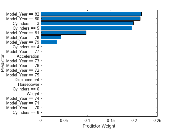
Figure contains an axes object. The axes object with xlabel Predictor Weight, ylabel Predictor contains an object of type bar.

The predictor weights indicate that multiple dummy variables for the categorical predictors Model_Year and Cylinders are important.

Specify Query Point

Find the observations whose MPG values are smaller than the 0.25 quantile of MPG. From the subset, choose four query points that do not include missing values.

rng('default') % For reproducibility
idx_subset = find(MPG < quantile(MPG,0.25));
tbl_subset = tbl(idx_subset,:);
queryPoint = datasample(rmmissing(tbl_subset),4,'Replace',false)

queryPoint=4×6 table
    Acceleration    Cylinders    Displacement    Horsepower    Model_Year    Weight
    ____________    _________    ____________    __________    __________    ______

        13.2            8            318            150            76         3940 
        14.9            8            302            130            77         4295 
          14            8            360            215            70         4615 
        13.7            8            318            145            77         4140

Use LIME with Tree Simple Models

Explain the predictions for the query points using lime with decision tree simple models. lime generates a synthetic data set and fits a simple model to the synthetic data set.

Create a lime object using tbl_subset so that lime generates a synthetic data set using the subset instead of the entire data set. Specify SimpleModelType as 'tree' to use a decision tree simple model.

explainer_lime = lime(blackbox,tbl_subset,'SimpleModelType','tree');

Fit simple models for the four query points by using the object function fit. Specify the third input (the number of important predictors to use in the simple model) as 6. With this setting, the software specifies the maximum number of decision splits (or branch nodes) as 6 so that the fitted decision tree uses at most all predictors.

explainer_lime1 = fit(explainer_lime,queryPoint(1,:),6);
explainer_lime2 = fit(explainer_lime,queryPoint(2,:),6);
explainer_lime3 = fit(explainer_lime,queryPoint(3,:),6);
explainer_lime4 = fit(explainer_lime,queryPoint(4,:),6);

Plot the predictor importance by using the object function plot.

tiledlayout(2,2)
nexttile
plot(explainer_lime1)
nexttile
plot(explainer_lime2)
nexttile
plot(explainer_lime3)
nexttile
plot(explainer_lime4)

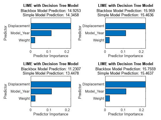
All simple models identify Displacement, Model_Year, and Weight as important predictors.

Compute Shapley Values

The Shapley value of a predictor for a query point explains the deviation of the predicted response for the query point from the average response, due to the predictor. Create a shapley object for the model blackbox using tbl_subset so that shapley computes the expected contribution based on the observations in tbl_subset.

explainer_shapley = shapley(blackbox,tbl_subset);

Compute the Shapley values for the query points by using the object function fit.

explainer_shapley1 = fit(explainer_shapley,queryPoint(1,:));
explainer_shapley2 = fit(explainer_shapley,queryPoint(2,:));
explainer_shapley3 = fit(explainer_shapley,queryPoint(3,:));
explainer_shapley4 = fit(explainer_shapley,queryPoint(4,:));

Plot the Shapley values by using the object function plot.

tiledlayout(2,2)
nexttile
plot(explainer_shapley1)
nexttile
plot(explainer_shapley2)
nexttile
plot(explainer_shapley3)
nexttile
plot(explainer_shapley4)

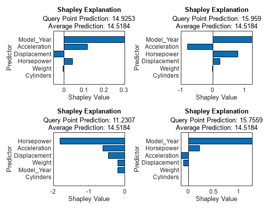
Model_Year is the most important predictor for the first, second, and fourth query points, and the Shapley values of Model_Year are positive for the three query points. The Model_Year variable value is 76 or 77 for these three points, and the value for the third query point is 70. According to the Shapley values for the four query points, a small Model_Year value leads to a decrease in the predicted response, and a large Model_Year value leads to an increase in the predicted response compared to the average.

Create Partial Dependence Plot (PDP)

A PDP plot shows the averaged relationships between the predictor and the predicted response in the trained model. Create a PDP for Model_Year, which the other interpretability tools identify as an important predictor. Pass tbl_subset to plotPartialDependence so that the function computes the expectation of the predicted responses using only the samples in tbl_subset.

figure
plotPartialDependence(blackbox,'Model_Year',tbl_subset)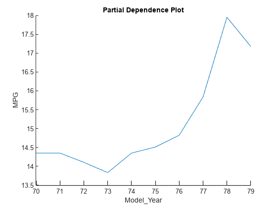

Figure contains an axes object. The axes object with title Partial Dependence Plot, xlabel M o d e l indexOf Y baseline e a r Model_Year, ylabel MPG contains an object of type line.

The plot shows the same trend identified by the Shapley values for the four query points. The predicted response (MPG) value increases as the Model_Year value increases.

References

[1] Ribeiro, Marco Tulio, S. Singh, and C. Guestrin. "'Why Should I Trust You?': Explaining the Predictions of Any Classifier." In Proceedings of the 22nd ACM SIGKDD International Conference on Knowledge Discovery and Data Mining, 1135–44. San Francisco, California: ACM, 2016.

[2] Lundberg, Scott M., and S. Lee. "A Unified Approach to Interpreting Model Predictions." Advances in Neural Information Processing Systems 30 (2017): 4765–774.

[3] Aas, Kjersti, Martin Jullum, and Anders Løland. "Explaining Individual Predictions When Features Are Dependent: More Accurate Approximations to Shapley Values." Artificial Intelligence 298 (September 2021).

[4] Lundberg, Scott M., G. Erion, H. Chen, et al. "From Local Explanations to Global Understanding with Explainable AI for Trees." Nature Machine Intelligence 2 (January 2020): 56–67.

[5] Friedman, Jerome. H. “Greedy Function Approximation: A Gradient Boosting Machine.” The Annals of Statistics 29, no. 5 (2001): 1189-1232.

[6] Goldstein, Alex, Adam Kapelner, Justin Bleich, and Emil Pitkin. “Peeking Inside the Black Box: Visualizing Statistical Learning with Plots of Individual Conditional Expectation.” Journal of Computational and Graphical Statistics 24, no. 1 (January 2, 2015): 44–65.