Main Content

plotPartialDependence

Create partial dependence plot (PDP) and individual conditional expectation (ICE) plots

Description

example

plotPartialDependence(RegressionMdl,Vars) computes and plots the partial dependence between the predictor variables listed in Vars and the responses predicted by using the regression model RegressionMdl, which contains predictor data.

  • If you specify one variable in Vars, the function creates a line plot of the partial dependence against the variable.

  • If you specify two variables in Vars, the function creates a surface plot of the partial dependence against the two variables.

example

plotPartialDependence(ClassificationMdl,Vars,Labels) computes and plots the partial dependence between the predictor variables listed in Vars and the scores for the classes specified in Labels by using the classification model ClassificationMdl, which contains predictor data.

  • If you specify one variable in Vars, the function creates a line plot of the partial dependence against the variable for each class in Labels.

  • If you specify two variables in Vars, the function creates a surface plot of the partial dependence against the two variables. You must specify one class in Labels.

example

plotPartialDependence(___,Data) uses new predictor data Data. You can specify Data in addition to any of the input argument combinations in the previous syntaxes.

example

plotPartialDependence(fun,Vars,Data) computes and plots the partial dependence between the predictor variables listed in Vars and the outputs returned by the custom model fun, using the predictor data Data.

  • If you specify one variable in Vars, the function creates a line plot of the partial dependence against the variable for each column of the output returned by fun.

  • If you specify two variables in Vars, the function creates a surface plot of the partial dependence against the two variables. When you specify two variables, fun must return a column vector or you must specify which output column to use by setting the OutputColumns name-value argument.

example

plotPartialDependence(___,Name,Value) uses additional options specified by one or more name-value arguments. For example, if you specify "Conditional","absolute", the plotPartialDependence function creates a figure including a PDP, a scatter plot of the selected predictor variable and predicted responses or scores, and an ICE plot for each observation.

example

ax = plotPartialDependence(___) returns the axes of the plot.

Examples

collapse all

Train a regression tree using the carsmall data set, and create a PDP that shows the relationship between a feature and the predicted responses in the trained regression tree.

Load the carsmall data set.

load carsmall

Specify Weight, Cylinders, and Horsepower as the predictor variables (X), and MPG as the response variable (Y).

X = [Weight,Cylinders,Horsepower];
Y = MPG;

Train a regression tree using X and Y.

Mdl = fitrtree(X,Y);

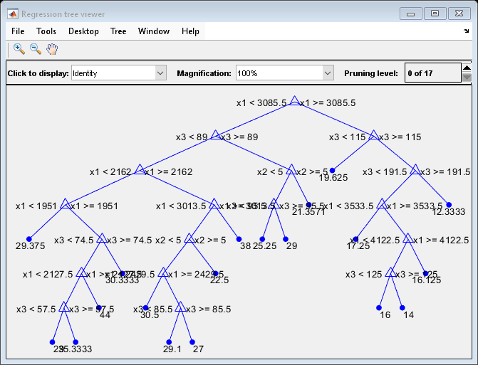
View a graphical display of the trained regression tree.

view(Mdl,"Mode","graph")

Figure Regression tree viewer contains an axes object and other objects of type uimenu, uicontrol. The axes object contains 60 objects of type line, text. One or more of the lines displays its values using only markers

Create a PDP of the first predictor variable, Weight.

plotPartialDependence(Mdl,1)

Figure contains an axes object. The axes object with title Partial Dependence Plot, xlabel x1, ylabel Y contains an object of type line.

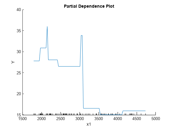
The plotted line represents averaged partial relationships between Weight (labeled as x1) and MPG (labeled as Y) in the trained regression tree Mdl. The x-axis minor ticks represent the unique values in x1.

The regression tree viewer shows that the first decision is whether x1 is smaller than 3085.5. The PDP also shows a large change near x1 = 3085.5. The tree viewer visualizes each decision at each node based on predictor variables. You can find several nodes split based on the values of x1, but determining the dependence of Y on x1 is not easy. However, the plotPartialDependence plots average predicted responses against x1, so you can clearly see the partial dependence of Y on x1.

The labels x1 and Y are the default values of the predictor names and the response name. You can modify these names by specifying the name-value arguments PredictorNames and ResponseName when you train Mdl using fitrtree. You can also modify axis labels by using the xlabel and ylabel functions.

Train a naive Bayes classification model with the fisheriris data set, and create a PDP that shows the relationship between the predictor variable and the predicted scores (posterior probabilities) for multiple classes.

Load the fisheriris data set, which contains species (species) and measurements (meas) on sepal length, sepal width, petal length, and petal width for 150 iris specimens. The data set contains 50 specimens from each of three species: setosa, versicolor, and virginica.

load fisheriris

Train a naive Bayes classification model with species as the response and meas as predictors.

Mdl = fitcnb(meas,species);

Create a PDP of the scores predicted by Mdl for all three classes of species against the third predictor variable x3. Specify the class labels by using the ClassNames property of Mdl.

plotPartialDependence(Mdl,3,Mdl.ClassNames);

Figure contains an axes object. The axes object with title Partial Dependence Plot, xlabel x3, ylabel Scores contains 3 objects of type line. These objects represent setosa, versicolor, virginica.

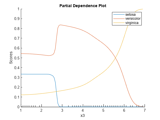
According to this model, the probability of virginica increases with x3. The probability of setosa is about 0.33, from where x3 is 0 to around 2.5, and then the probability drops to almost 0.

Train a Gaussian process regression model using generated sample data where a response variable includes interactions between predictor variables. Then, create ICE plots that show the relationship between a feature and the predicted responses for each observation.

Generate sample predictor data x1 and x2.

rng("default") % For reproducibility
n = 200;
x1 = rand(n,1)*2-1;
x2 = rand(n,1)*2-1;

Generate response values that include interactions between x1 and x2.

Y = x1-2*x1.*(x2>0)+0.1*rand(n,1);

Create a Gaussian process regression model using [x1 x2] and Y.

Mdl = fitrgp([x1 x2],Y);

Create a figure including a PDP (red line) for the first predictor x1, a scatter plot (circle markers) of x1 and predicted responses, and a set of ICE plots (gray lines) by specifying Conditional as "centered".

plotPartialDependence(Mdl,1,"Conditional","centered")

Figure contains an axes object. The axes object with title Individual Conditional Expectation Plot, xlabel x1, ylabel Y contains 202 objects of type line, scatter.

When Conditional is "centered", plotPartialDependence offsets plots so that all plots start from zero, which is helpful in examining the cumulative effect of the selected feature.

A PDP finds averaged relationships, so it does not reveal hidden dependencies especially when responses include interactions between features. However, the ICE plots clearly show two different dependencies of responses on x1.

Train an ensemble of classification models and create two PDPs, one using the training data set and the other using a new data set.

Load the census1994 data set, which contains US yearly salary data, categorized as <=50K or >50K, and several demographic variables.

load census1994

Extract a subset of variables to analyze from the tables adultdata and adulttest.

X = adultdata(:,["age","workClass","education_num","marital_status","race", ...
   "sex","capital_gain","capital_loss","hours_per_week","salary"]);
Xnew = adulttest(:,["age","workClass","education_num","marital_status","race", ...
   "sex","capital_gain","capital_loss","hours_per_week","salary"]);

Train an ensemble of classifiers with salary as the response and the remaining variables as predictors by using the function fitcensemble. For binary classification, fitcensemble aggregates 100 classification trees using the LogitBoost method.

Mdl = fitcensemble(X,"salary");

Inspect the class names in Mdl.

Mdl.ClassNames
ans = 2x1 categorical
     <=50K 
     >50K 

Create a partial dependence plot of the scores predicted by Mdl for the second class of salary (>50K) against the predictor age using the training data.

plotPartialDependence(Mdl,"age",Mdl.ClassNames(2))

Figure contains an axes object. The axes object with title Partial Dependence Plot, xlabel age, ylabel Score of class >50K contains an object of type line.

Create a PDP of the scores for class >50K against age using new predictor data from the table Xnew.

plotPartialDependence(Mdl,"age",Mdl.ClassNames(2),Xnew)

Figure contains an axes object. The axes object with title Partial Dependence Plot, xlabel age, ylabel Score of class >50K contains an object of type line.

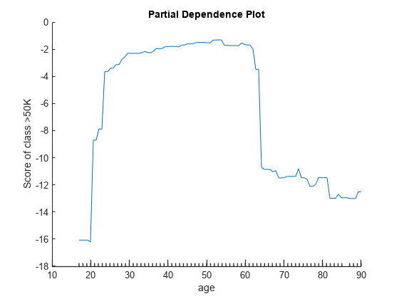
The two plots show similar shapes for the partial dependence of the predicted score of high salary (>50K) on age. Both plots indicate that the predicted score of high salary rises fast until the age of 30, then stays almost flat until the age of 60, and then drops fast. However, the plot based on the new data produces slightly higher scores for ages over 65.

Create a PDP to analyze relationships between predictors and anomaly scores for an isolationForest object. You cannot pass an isolationForest object directly to the plotPartialDependence function. Instead, define a custom function that returns anomaly scores for the object, and then pass the function to plotPartialDependence.

Load the 1994 census data stored in census1994.mat. The data set consists of demographic data from the US Census Bureau.

load census1994

census1994 contains the two data sets adultdata and adulttest.

Train an isolation forest model for adulttest. The function iforest returns an IsolationForest object.

rng("default") % For reproducibility
Mdl = iforest(adulttest);

Define the custom function myAnomalyScores, which returns anomaly scores computed by the isanomaly function of IsolationForest; the custom function definition appears at the end of this example.

Create a PDP of the anomaly scores against the variable age for the adulttest data set. plotPartialDependence accepts a custom model in the form of a function handle. The function represented by the function handle must accept predictor data and return a column vector or matrix with one row for each observation. Specify the custom model as @(tbl)myAnomalyScores(Mdl,tbl) so that the custom function uses the trained model Mdl and accepts predictor data.

plotPartialDependence(@(tbl)myAnomalyScores(Mdl,tbl),"age",adulttest)
xlabel("Age")
ylabel("Anomaly Score")

Figure contains an axes object. The axes object with title Partial Dependence Plot, xlabel Age, ylabel Anomaly Score contains an object of type line.

Custom Function myAnomalyScores

function scores = myAnomalyScores(Mdl,tbl)
[~,scores] = isanomaly(Mdl,tbl);
end

Train a regression ensemble using the carsmall data set, and create a PDP plot and ICE plots for each predictor variable using a new data set, carbig. Then, compare the figures to analyze the importance of predictor variables. Also, compare the results with the estimates of predictor importance returned by the predictorImportance function.

Load the carsmall data set.

load carsmall

Specify Weight, Cylinders, Horsepower, and Model_Year as the predictor variables (X), and MPG as the response variable (Y).

X = [Weight,Cylinders,Horsepower,Model_Year];
Y = MPG;

Train a regression ensemble using X and Y.

Mdl = fitrensemble(X,Y, ...
    "PredictorNames",["Weight","Cylinders","Horsepower","Model Year"], ...
    "ResponseName","MPG");

Create the importance of predictor variables by using the plotPartialDependence and predictorImportance functions. The plotPartialDependence function visualizes the relationships between a selected predictor and predicted responses. predictorImportance summarizes the importance of a predictor with a single value.

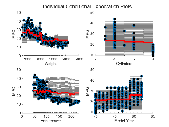
Create a figure including a PDP plot (red line) and ICE plots (gray lines) for each predictor by using plotPartialDependence and specifying "Conditional","absolute". Each figure also includes a scatter plot (circle markers) of the selected predictor and predicted responses. Also, load the carbig data set and use it as new predictor data, Xnew. When you provide Xnew, the plotPartialDependence function uses Xnew instead of the predictor data in Mdl.

load carbig
Xnew = [Weight,Cylinders,Horsepower,Model_Year];

figure
t = tiledlayout(2,2,"TileSpacing","compact");
title(t,"Individual Conditional Expectation Plots")

for i = 1 : 4
    nexttile
    plotPartialDependence(Mdl,i,Xnew,"Conditional","absolute")
    title("")
end

Figure contains 4 axes objects. Axes object 1 with xlabel Weight, ylabel MPG contains 408 objects of type line, scatter. Axes object 2 with xlabel Cylinders, ylabel MPG contains 408 objects of type line, scatter. Axes object 3 with xlabel Horsepower, ylabel MPG contains 408 objects of type line, scatter. Axes object 4 with xlabel Model Year, ylabel MPG contains 408 objects of type line, scatter.

Compute estimates of predictor importance by using predictorImportance. This function sums changes in the mean squared error (MSE) due to splits on every predictor, and then divides the sum by the number of branch nodes.

imp = predictorImportance(Mdl);
figure
bar(imp)
title("Predictor Importance Estimates")
ylabel("Estimates")
xlabel("Predictors")
ax = gca;
ax.XTickLabel = Mdl.PredictorNames;

Figure contains an axes object. The axes object with title Predictor Importance Estimates, xlabel Predictors, ylabel Estimates contains an object of type bar.

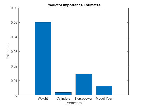
The variable Weight has the most impact on MPG according to predictor importance. The PDP of Weight also shows that MPG has high partial dependence on Weight. The variable Cylinders has the least impact on MPG according to predictor importance. The PDP of Cylinders also shows that MPG does not change much depending on Cylinders.

Train a generalized additive model (GAM) with both linear and interaction terms for predictors. Then, create a PDP with both linear and interaction terms and a PDP with only linear terms. Specify whether to include interaction terms when creating the PDPs.

Load the ionosphere data set. This data set has 34 predictors and 351 binary responses for radar returns, either bad ('b') or good ('g').

load ionosphere

Train a GAM using the predictors X and class labels Y. A recommended practice is to specify the class names. Specify to include the 10 most important interaction terms.

Mdl = fitcgam(X,Y,"ClassNames",{'b','g'},"Interactions",10);

Mdl is a ClassificationGAM model object.

List the interaction terms in Mdl.

Mdl.Interactions
ans = 10×2

     1     5
     7     8
     6     7
     5     6
     5     7
     5     8
     3     5
     4     7
     1     7
     4     5

Each row of Interactions represents one interaction term and contains the column indexes of the predictor variables for the interaction term.

Find the most frequent predictor in the interaction terms.

mode(Mdl.Interactions,"all")
ans = 5

The most frequent predictor in the interaction terms is the 5th predictor (x5). Create PDPs for the 5th predictor. To exclude interaction terms from the computation, specify "IncludeInteractions",false for the second PDP.

plotPartialDependence(Mdl,5,Mdl.ClassNames(1))
hold on
plotPartialDependence(Mdl,5,Mdl.ClassNames(1),"IncludeInteractions",false)
grid on
legend("Linear and interaction terms","Linear terms only")
title("PDPs of Posterior Probabilities for 5th Predictor")
hold off

Figure contains an axes object. The axes object with title PDPs of Posterior Probabilities for 5th Predictor, xlabel x5, ylabel Score of class b contains 2 objects of type line. These objects represent Linear and interaction terms, Linear terms only.

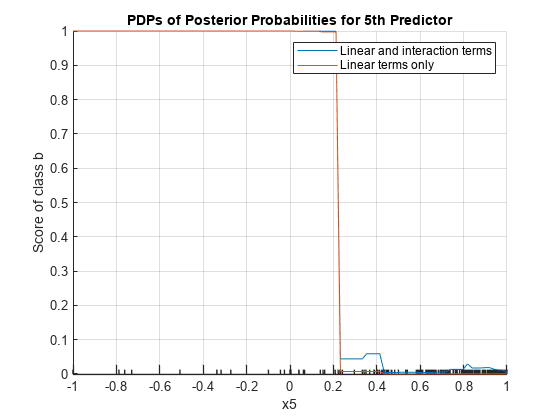
The plot shows that the partial dependence of the scores (posterior probabilities) on x5 varies depending on whether the model includes the interaction terms, especially where x5 is between 0.2 and 0.45.

Train a support vector machine (SVM) regression model using the carsmall data set, and create a PDP for two predictor variables. Then, extract partial dependence estimates from the output of plotPartialDependence. Alternatively, you can get the partial dependence values by using the partialDependence function.

Load the carsmall data set.

load carsmall

Specify Weight, Cylinders, Displacement, and Horsepower as the predictor variables (Tbl).

Tbl = table(Weight,Cylinders,Displacement,Horsepower);

Construct an SVM regression model using Tbl and the response variable MPG. Use a Gaussian kernel function with an automatic kernel scale.

Mdl = fitrsvm(Tbl,MPG,"ResponseName","MPG", ...
    "CategoricalPredictors","Cylinders","Standardize",true, ...
    "KernelFunction","gaussian","KernelScale","auto");

Create a PDP that visualizes partial dependence of predicted responses (MPG) on the predictor variables Weight and Cylinders. Specify query points to compute the partial dependence for Weight by using the QueryPoints name-value argument. You cannot specify the QueryPoints value for Cylinders because it is a categorical variable. plotPartialDependence uses all categorical values.

pt = linspace(min(Weight),max(Weight),50)';
ax = plotPartialDependence(Mdl,["Weight","Cylinders"],"QueryPoints",{pt,[]});
view(140,30) % Modify the viewing angle

Figure contains an axes object. The axes object with title Partial Dependence Plot, xlabel Weight, ylabel Cylinders contains an object of type surface.

The PDP shows an interaction effect between Weight and Cylinders. The partial dependence of MPG on Weight changes depending on the value of Cylinders.

Extract the estimated partial dependence of MPG on Weight and Cylinders. The XData, YData, and ZData values of ax.Children are x-axis values (the first selected predictor values), y-axis values (the second selected predictor values), and z-axis values (the corresponding partial dependence values), respectively.

xval = ax.Children.XData;
yval = ax.Children.YData;
zval = ax.Children.ZData;

Alternatively, you can get the partial dependence values by using the partialDependence function.

[pd,x,y] = partialDependence(Mdl,["Weight","Cylinders"],"QueryPoints",{pt,[]});

pd contains the partial dependence values for the query points x and y.

If you specify Conditional as "absolute", plotPartialDependence creates a figure including a PDP, a scatter plot, and a set of ICE plots. ax.Children(1) and ax.Children(2) correspond to the PDP and scatter plot, respectively. The remaining elements of ax.Children correspond to the ICE plots. The XData and YData values of ax.Children(i) are x-axis values (the selected predictor values) and y-axis values (the corresponding partial dependence values), respectively.

Input Arguments

collapse all

Regression model, specified as a full or compact regression model object, as given in the following tables of supported models.

ModelFull or Compact Model Object
Generalized linear modelGeneralizedLinearModel, CompactGeneralizedLinearModel
Generalized linear mixed-effect modelGeneralizedLinearMixedModel
Linear regressionLinearModel, CompactLinearModel
Linear mixed-effect modelLinearMixedModel
Nonlinear regressionNonLinearModel
Ensemble of regression modelsRegressionEnsemble, RegressionBaggedEnsemble, CompactRegressionEnsemble
Generalized additive model (GAM)RegressionGAM, CompactRegressionGAM
Gaussian process regressionRegressionGP, CompactRegressionGP
Gaussian kernel regression model using random feature expansionRegressionKernel
Linear regression for high-dimensional dataRegressionLinear
Neural network regression modelRegressionNeuralNetwork, CompactRegressionNeuralNetwork
Support vector machine (SVM) regressionRegressionSVM, CompactRegressionSVM
Regression treeRegressionTree, CompactRegressionTree
Bootstrap aggregation for ensemble of decision treesTreeBagger, CompactTreeBagger

If RegressionMdl is a model object that does not contain predictor data (for example, a compact model), you must provide the input argument Data.

plotPartialDependence does not support a model object trained with a sparse matrix. When you train a model, use a full numeric matrix or table for predictor data where rows correspond to individual observations.

Classification model, specified as a full or compact classification model object, as given in the following table of supported models.

ModelFull or Compact Model Object
Discriminant analysis classifierClassificationDiscriminant, CompactClassificationDiscriminant
Multiclass model for support vector machines or other classifiersClassificationECOC, CompactClassificationECOC
Ensemble of learners for classificationClassificationEnsemble, CompactClassificationEnsemble, ClassificationBaggedEnsemble
Generalized additive model (GAM)ClassificationGAM, CompactClassificationGAM
Gaussian kernel classification model using random feature expansionClassificationKernel
k-nearest neighbor classifierClassificationKNN
Linear classification modelClassificationLinear
Multiclass naive Bayes modelClassificationNaiveBayes, CompactClassificationNaiveBayes
Neural network classifierClassificationNeuralNetwork, CompactClassificationNeuralNetwork
Support vector machine (SVM) classifier for one-class and binary classificationClassificationSVM, CompactClassificationSVM
Binary decision tree for multiclass classificationClassificationTree, CompactClassificationTree
Bagged ensemble of decision treesTreeBagger, CompactTreeBagger
Multinomial regression modelMultinomialRegression

If ClassificationMdl is a model object that does not contain predictor data (for example, a compact model), you must provide the input argument Data.

plotPartialDependence does not support a model object trained with a sparse matrix. When you train a model, use a full numeric matrix or table for predictor data where rows correspond to individual observations.

Custom model, specified as a function handle. The function handle fun must represent a function that accepts the predictor data Data and returns an output in the form of a column vector or matrix. Each row of the output must correspond to each observation (row) in the predictor data.

By default, plotPartialDependence uses all output columns of fun for the partial dependence computation. You can specify which output columns to use by setting the OutputColumns name-value argument.

If the predictor data (Data) is in a table, plotPartialDependence assumes that a variable is categorical if it is a logical vector, categorical vector, character array, string array, or cell array of character vectors. If the predictor data is a matrix, plotPartialDependence assumes that all predictors are continuous. To identify any other predictors as categorical predictors, specify them by using the CategoricalPredictors name-value argument.

Data Types: function_handle

Predictor variables, specified as a vector of positive integers, character vector, string scalar, string array, or cell array of character vectors. You can specify one or two predictor variables, as shown in the following tables.

One Predictor Variable

ValueDescription
positive integerIndex value corresponding to the column of the predictor data.
character vector or string scalar

Name of the predictor variable. The name must match the entry in the PredictorNames property for RegressionMdl and ClassificationMdl or the variable name of Data in a table for a custom model fun.

Two Predictor Variables

ValueDescription
vector of two positive integersIndex values corresponding to the columns of the predictor data.
string array or cell array of character vectors

Names of the predictor variables. Each element in the array is the name of a predictor variable. The names must match the entries in the PredictorNames property for RegressionMdl and ClassificationMdl or the variable names of Data in a table for a custom model fun.

If you specify two predictor variables, you must specify one class in Labels for ClassificationMdl or specify one output column in OutputColumns for a custom model fun.

Example: ["x1","x3"]

Data Types: single | double | char | string | cell

Class labels, specified as a categorical or character array, logical or numeric vector, or cell array of character vectors. The values and data types in Labels must match those of the class names in the ClassNames property of ClassificationMdl (ClassificationMdl.ClassNames).

  • You can specify multiple class labels only when you specify one variable in Vars and specify Conditional as "none" (default).

  • Use partialDependence if you want to compute the partial dependence for two variables and multiple class labels in one function call.

This argument is valid only when you specify a classification model object ClassificationMdl.

Example: ["red","blue"]

Example: ClassificationMdl.ClassNames([1 3]) specifies Labels as the first and third classes in ClassificationMdl.

Data Types: single | double | logical | char | cell | categorical

Predictor data, specified as a numeric matrix or table. Each row of Data corresponds to one observation, and each column corresponds to one variable.

For both a regression model (RegressionMdl) and a classification model (ClassificationMdl), Data must be consistent with the predictor data that trained the model, stored in either the X or Variables property.

  • If you trained the model using a numeric matrix, then Data must be a numeric matrix. The variables that make up the columns of Data must have the same number and order as the predictor variables that trained the model.

  • If you trained the model using a table (for example, Tbl), then Data must be a table. All predictor variables in Data must have the same variable names and data types as the names and types in Tbl. However, the column order of Data does not need to correspond to the column order of Tbl.

  • Data must not be sparse.

If you specify a regression or classification model that does not contain predictor data, you must provide Data. If the model is a full model object that contains predictor data and you specify the Data argument, then plotPartialDependence ignores the predictor data in the model and uses Data only.

If you specify a custom model fun, you must provide Data.

Data Types: single | double | table

Name-Value Arguments

Specify optional pairs of arguments as Name1=Value1,...,NameN=ValueN, where Name is the argument name and Value is the corresponding value. Name-value arguments must appear after other arguments, but the order of the pairs does not matter.

Before R2021a, use commas to separate each name and value, and enclose Name in quotes.

Example: plotPartialDependence(Mdl,Vars,Data,"NumObservationsToSample",100,"UseParallel",true) creates a PDP by using 100 sampled observations in Data and executing for-loop iterations in parallel.

Plot type, specified as "none", "absolute", or "centered".

ValueDescription
"none"

plotPartialDependence creates a PDP. The plot type depends on the number of predictor variables specified in Vars.

  • One predictor variable — plotPartialDependence creates a 2-D line plot of the partial dependence. If you provide a classification model (ClassificationMdl), the function creates a line plot for each class label specified in Labels. If you provide a custom model (fun), the function creates a line plot for each column of the output returned by fun. You can specify which output columns to use by setting the OutputColumns name-value argument.

  • Two predictor variables — plotPartialDependence creates a surface plot of partial dependence against the two variables. For a classification model, you must specify one class label in Labels. For a custom model, you must provide a model that returns a column vector or specify which output column to use by setting the OutputColumns name-value argument.

"absolute"

plotPartialDependence creates a figure that includes three types of plots:

  • PDP with a red line

  • Scatter plot of the selected predictor variable and predicted responses or scores with circle markers

  • ICE plot for each observation with a gray line

To use the "absolute" option, you must specify one predictor variable in Vars. In addition, for a classification model, you must specify one class label in Labels. For a custom model, you must provide a model that returns a column vector or specify which output column to use by setting the OutputColumns name-value argument.

"centered"

plotPartialDependence creates a figure that includes the same three types of plots as "absolute". The function offsets plots so that all plots start from zero.

To use the "centered" option, you must specify one predictor variable in Vars. In addition, for a classification model, you must specify one class label in Labels. For a custom model, you must provide a model that returns a column vector or specify which output column to use by setting the OutputColumns name-value argument.

Example: "Conditional","absolute"

Flag to include interaction terms of the generalized additive model (GAM) in the partial dependence computation, specified as true or false. This argument is valid only for a GAM. That is, you can specify this argument only when RegressionMdl is RegressionGAM or CompactRegressionGAM, or ClassificationMdl is ClassificationGAM or CompactClassificationGAM.

The default IncludeInteractions value is true if the model contains interaction terms. The value must be false if the model does not contain interaction terms.

Example: "IncludeInteractions",false

Data Types: logical

Flag to include an intercept term of the generalized additive model (GAM) in the partial dependence computation, specified as true or false. This argument is valid only for a GAM. That is, you can specify this argument only when RegressionMdl is RegressionGAM or CompactRegressionGAM, or ClassificationMdl is ClassificationGAM or CompactClassificationGAM.

Example: "IncludeIntercept",false

Data Types: logical

Number of observations to sample, specified as a positive integer. The default value is the number of total observations in Data or the model (RegressionMdl or ClassificationMdl). If you specify a value larger than the number of total observations, then plotPartialDependence uses all observations.

plotPartialDependence samples observations without replacement by using the datasample function and uses the sampled observations to compute partial dependence.

plotPartialDependence displays minor tick marks at the unique values of the sampled observations.

If you specify Conditional as either "absolute" or "centered", plotPartialDependence creates a figure including an ICE plot for each sampled observation.

Example: "NumObservationsToSample",100

Data Types: single | double

Axes in which to plot, specified as an axes object. If you do not specify the axes and if the current axes are Cartesian, then plotPartialDependence uses the current axes (gca). If axes do not exist, plotPartialDependence plots in a new figure.

Example: "Parent",ax

Points to compute partial dependence for numeric predictors, specified as a numeric column vector, a numeric two-column matrix, or a cell array of two numeric column vectors.

  • If you select one predictor variable in Vars, use a numeric column vector.

  • If you select two predictor variables in Vars:

    • Use a numeric two-column matrix to specify the same number of points for each predictor variable.

    • Use a cell array of two numeric column vectors to specify a different number of points for each predictor variable.

The default value is a numeric column vector or a numeric two-column matrix, depending on the number of selected predictor variables. Each column contains 100 evenly spaced points between the minimum and maximum values of the sampled observations for the corresponding predictor variable.

If Conditional is "absolute" or "centered", then the software adds the predictor data values (Data or predictor data in RegressionMdl or ClassificationMdl) of the selected predictors to the query points.

You cannot modify QueryPoints for a categorical variable. The plotPartialDependence function uses all categorical values in the selected variable.

If you select one numeric variable and one categorical variable, you can specify QueryPoints for a numeric variable by using a cell array consisting of a numeric column vector and an empty array.

Example: "QueryPoints",{pt,[]}

Data Types: single | double | cell

Flag to run in parallel, specified as true or false. If you specify "UseParallel",true, the plotPartialDependence function executes for-loop iterations by using parfor when predicting responses or scores for each observation and averaging them. The loop runs in parallel when you have Parallel Computing Toolbox™.

Example: "UseParallel",true

Data Types: logical

Categorical predictors list for the custom model fun, specified as one of the values in this table.

ValueDescription
Vector of positive integers

Each entry in the vector is an index value indicating that the corresponding predictor is categorical. The index values are between 1 and p, where p is the number of variables in Data.

Logical vector

A true entry means that the corresponding predictor is categorical. The length of the vector is p.

Character matrixEach row of the matrix is the name of a predictor variable. The names must match the variable names of the predictor data Data in a table. Pad the names with extra blanks so each row of the character matrix has the same length.
String array or cell array of character vectorsEach element in the array is the name of a predictor variable. The names must match the variable names of the predictor data Data in a table.
"all"All predictors are categorical.

By default, if the predictor data Data is in a table, plotPartialDependence assumes that a variable is categorical if it is a logical vector, categorical vector, character array, string array, or cell array of character vectors. If the predictor data is a matrix, plotPartialDependence assumes that all predictors are continuous. To identify any other predictors as categorical predictors, specify them by using the CategoricalPredictors name-value argument.

This argument is valid only when you specify a custom model by using fun.

Example: "CategoricalPredictors","all"

Data Types: single | double | logical | char | string | cell

Output columns of the custom model fun to use for the partial dependence computation, specified as one of the values in this table.

ValueDescription
Vector of positive integers

Each entry in the vector is an index value indicating that plotPartialDependence uses the corresponding output column for the partial dependence computation. The index values are between 1 and q, where q is the number of columns in the output matrix returned by the custom model fun.

Logical vector

A true entry means that plotPartialDependence uses the corresponding output column for the partial dependence computation. The length of the vector is q.

"all"plotPartialDependence uses all output columns for the partial dependence computation.

  • You can specify multiple output columns only when you specify one variable in Vars and specify Conditional as "none" (default).

  • Use partialDependence if you want to compute the partial dependence for two variables and multiple output columns in one function call.

This argument is valid only when you specify a custom model by using fun.

Example: "OutputColumns",[1 2]

Data Types: single | double | logical | char | string

Output Arguments

collapse all

Axes of the plot, returned as an axes object. For details on how to modify the appearance of the axes and extract data from plots, see Axes Appearance and Extract Partial Dependence Estimates from Plots.

More About

collapse all

Partial Dependence for Regression Models

Partial dependence[1] represents the relationships between predictor variables and predicted responses in a trained regression model. plotPartialDependence computes the partial dependence of predicted responses on a subset of predictor variables by marginalizing over the other variables.

Consider partial dependence on a subset XS of the whole predictor variable set X = {x1, x2, …, xm}. A subset XS includes either one variable or two variables: XS = {xS1} or XS = {xS1, xS2}. Let XC be the complementary set of XS in X. A predicted response f(X) depends on all variables in X:

f(X) = f(XS, XC).

The partial dependence of predicted responses on XS is defined by the expectation of predicted responses with respect to XC:

fS(XS)=EC[f(XS,XC)]=f(XS,XC)pC(XC)dXC,

where pC(XC) is the marginal probability of XC, that is, pC(XC)p(XS,XC)dXS. Assuming that each observation is equally likely, and the dependence between XS and XC and the interactions of XS and XC in responses is not strong, plotPartialDependence estimates the partial dependence by using observed predictor data as follows:

fS(XS)1Ni=1Nf(XS,XiC),(1)

where N is the number of observations and Xi = (XiS, XiC) is the ith observation.

When you call the plotPartialDependence function, you can specify a trained model (f(·)) and select variables (XS) by using the input arguments RegressionMdl and Vars, respectively. plotPartialDependence computes the partial dependence at 100 evenly spaced points of XS or the points that you specify by using the QueryPoints name-value argument. You can specify the number (N) of observations to sample from given predictor data by using the NumObservationsToSample name-value argument.

Individual Conditional Expectation for Regression Models

An individual conditional expectation (ICE) [2], as an extension of partial dependence, represents the relationship between a predictor variable and the predicted responses for each observation. While partial dependence shows the averaged relationship between predictor variables and predicted responses, a set of ICE plots disaggregates the averaged information and shows an individual dependence for each observation.

plotPartialDependence creates an ICE plot for each observation. A set of ICE plots is useful to investigate heterogeneities of partial dependence originating from different observations. plotPartialDependence can also create ICE plots with any predictor data provided through the input argument Data. You can use this feature to explore predicted response space.

Consider an ICE plot for a selected predictor variable xS with a given observation XiC, where XS = {xS}, XC is the complementary set of XS in the whole variable set X, and Xi = (XiS, XiC) is the ith observation. The ICE plot corresponds to the summand of the summation in Equation 1:

fSi(XS)=f(XS,XiC).

plotPartialDependence plots fSi(XS) for each observation i when you specify Conditional as "absolute". If you specify Conditional as "centered", plotPartialDependence draws all plots after removing level effects due to different observations:

fSi,centered(XS)=f(XS,XiC)f(min(XS),XiC).

This subtraction ensures that each plot starts from zero, so that you can examine the cumulative effect of XS and the interactions between XS and XC.

Partial Dependence and ICE for Classification Models

In the case of classification models, plotPartialDependence computes the partial dependence and individual conditional expectation in the same way as for regression models, with one exception: instead of using the predicted responses from the model, the function uses the predicted scores for the classes specified in Labels.

Weighted Traversal Algorithm

The weighted traversal algorithm[1] is a method to estimate partial dependence for a tree-based model. The estimated partial dependence is the weighted average of response or score values corresponding to the leaf nodes visited during the tree traversal.

Let XS be a subset of the whole variable set X and XC be the complementary set of XS in X. For each XS value to compute partial dependence, the algorithm traverses a tree from the root (beginning) node down to leaf (terminal) nodes and finds the weights of leaf nodes. The traversal starts by assigning a weight value of one at the root node. If a node splits by XS, the algorithm traverses to the appropriate child node depending on the XS value. The weight of the child node becomes the same value as its parent node. If a node splits by XC, the algorithm traverses to both child nodes. The weight of each child node becomes a value of its parent node multiplied by the fraction of observations corresponding to each child node. After completing the tree traversal, the algorithm computes the weighted average by using the assigned weights.

For an ensemble of bagged trees, the estimated partial dependence is an average of the weighted averages over the individual trees.

Algorithms

For both a regression model (RegressionMdl) and a classification model (ClassificationMdl), plotPartialDependence uses a predict function to predict responses or scores. plotPartialDependence chooses the proper predict function according to the model and runs predict with its default settings. For details about each predict function, see the predict functions in the following two tables. If the specified model is a tree-based model (not including a boosted ensemble of trees) and Conditional is "none", then plotPartialDependence uses the weighted traversal algorithm instead of the predict function. For details, see Weighted Traversal Algorithm.

Regression Model Object

Model TypeFull or Compact Regression Model ObjectFunction to Predict Responses
Bootstrap aggregation for ensemble of decision treesCompactTreeBaggerpredict
Bootstrap aggregation for ensemble of decision treesTreeBaggerpredict
Ensemble of regression modelsRegressionEnsemble, RegressionBaggedEnsemble, CompactRegressionEnsemblepredict
Gaussian kernel regression model using random feature expansionRegressionKernelpredict
Gaussian process regressionRegressionGP, CompactRegressionGPpredict
Generalized additive modelRegressionGAM, CompactRegressionGAMpredict
Generalized linear mixed-effect modelGeneralizedLinearMixedModelpredict
Generalized linear modelGeneralizedLinearModel, CompactGeneralizedLinearModelpredict
Linear mixed-effect modelLinearMixedModelpredict
Linear regressionLinearModel, CompactLinearModelpredict
Linear regression for high-dimensional dataRegressionLinearpredict
Neural network regression modelRegressionNeuralNetwork, CompactRegressionNeuralNetworkpredict
Nonlinear regressionNonLinearModelpredict
Regression treeRegressionTree, CompactRegressionTreepredict
Support vector machineRegressionSVM, CompactRegressionSVMpredict

Classification Model Object

Model TypeFull or Compact Classification Model ObjectFunction to Predict Labels and Scores
Discriminant analysis classifierClassificationDiscriminant, CompactClassificationDiscriminantpredict
Multiclass model for support vector machines or other classifiersClassificationECOC, CompactClassificationECOCpredict
Ensemble of learners for classificationClassificationEnsemble, CompactClassificationEnsemble, ClassificationBaggedEnsemblepredict
Gaussian kernel classification model using random feature expansionClassificationKernelpredict
Generalized additive modelClassificationGAM, CompactClassificationGAMpredict
k-nearest neighbor modelClassificationKNNpredict
Linear classification modelClassificationLinearpredict
Naive Bayes modelClassificationNaiveBayes, CompactClassificationNaiveBayespredict
Neural network classifierClassificationNeuralNetwork, CompactClassificationNeuralNetworkpredict
Support vector machine for one-class and binary classificationClassificationSVM, CompactClassificationSVMpredict
Binary decision tree for multiclass classificationClassificationTree, CompactClassificationTreepredict
Bagged ensemble of decision treesTreeBagger, CompactTreeBaggerpredict

Alternative Functionality

  • partialDependence computes partial dependence without visualization. The function can compute partial dependence for two variables and multiple classes in one function call.

References

[1] Friedman, Jerome. H. “Greedy Function Approximation: A Gradient Boosting Machine.” The Annals of Statistics 29, no. 5 (2001): 1189-1232.

[2] Goldstein, Alex, Adam Kapelner, Justin Bleich, and Emil Pitkin. “Peeking Inside the Black Box: Visualizing Statistical Learning with Plots of Individual Conditional Expectation.” Journal of Computational and Graphical Statistics 24, no. 1 (January 2, 2015): 44–65.

[3] Hastie, Trevor, Robert Tibshirani, and Jerome Friedman. The Elements of Statistical Learning. New York, NY: Springer New York, 2001.

Extended Capabilities

Version History

Introduced in R2017b

expand all