Linear Regression

Prepare Data

To begin fitting a regression, put your data into a form that fitting functions expect. All regression techniques begin with input data in an array X and response data in a separate vector y, or input data in a table or dataset array tbl and response data as a column in tbl. Each row of the input data represents one observation. Each column represents one predictor (variable).

For a table or dataset array tbl, indicate the response variable with the 'ResponseVar' name-value pair:

mdl = fitlm(tbl,'ResponseVar','BloodPressure');

The response variable is the last column by default.

You can use numeric categorical predictors. A categorical predictor is one that takes values from a fixed set of possibilities.

For a numeric array X, indicate the categorical predictors using the 'Categorical' name-value pair. For example, to indicate that predictors 2 and 3 out of six are categorical:
```
mdl = fitlm(X,y,'Categorical',[2,3]);
% or equivalently
mdl = fitlm(X,y,'Categorical',logical([0 1 1 0 0 0]));
```
For a table or dataset array tbl, fitting functions assume that these data types are categorical:
- Logical vector
- Categorical vector
- Character array
- String array
If you want to indicate that a numeric predictor is categorical, use the 'Categorical' name-value pair.

Represent missing numeric data as NaN. To represent missing data for other data types, see Missing Group Values.

Dataset Array for Input and Response Data

To create a dataset array from an Excel^® spreadsheet:

ds = dataset('XLSFile','hospital.xls', ...
    'ReadObsNames',true);

To create a dataset array from workspace variables:

load carsmall
ds = dataset(MPG,Weight);
ds.Year = categorical(Model_Year);

Table for Input and Response Data

To create a table from an Excel spreadsheet:

tbl = readtable('hospital.xls', ...
    'ReadRowNames',true);

To create a table from workspace variables:

load carsmall
tbl = table(MPG,Weight);
tbl.Year = categorical(Model_Year);

Numeric Matrix for Input Data, Numeric Vector for Response

For example, to create numeric arrays from workspace variables:

load carsmall
X = [Weight Horsepower Cylinders Model_Year];
y = MPG;

To create numeric arrays from an Excel spreadsheet:

[X, Xnames] = xlsread('hospital.xls');
y = X(:,4); % response y is systolic pressure
X(:,4) = []; % remove y from the X matrix

Notice that the nonnumeric entries, such as sex, do not appear in X.

Choose a Fitting Method

There are three ways to fit a model to data:

Least-Squares Fit
Robust Fit
Stepwise Fit

Least-Squares Fit

Use fitlm to construct a least-squares fit of a model to the data. This method is best when you are reasonably certain of the model’s form, and mainly need to find its parameters. This method is also useful when you want to explore a few models. The method requires you to examine the data manually to discard outliers, though there are techniques to help (see Examine Quality and Adjust Fitted Model).

Robust Fit

Use fitlm with the RobustOpts name-value pair to create a model that is little affected by outliers. Robust fitting saves you the trouble of manually discarding outliers. However, step does not work with robust fitting. This means that when you use robust fitting, you cannot search stepwise for a good model.

Stepwise Fit

Use stepwiselm to find a model, and fit parameters to the model. stepwiselm starts from one model, such as a constant, and adds or subtracts terms one at a time, choosing an optimal term each time in a greedy fashion, until it cannot improve further. Use stepwise fitting to find a good model, which is one that has only relevant terms.

The result depends on the starting model. Usually, starting with a constant model leads to a small model. Starting with more terms can lead to a more complex model, but one that has lower mean squared error. See Compare Large and Small Stepwise Models.

You cannot use robust options along with stepwise fitting. So after a stepwise fit, examine your model for outliers (see Examine Quality and Adjust Fitted Model).

Choose a Model or Range of Models

There are several ways of specifying a model for linear regression. Use whichever you find most convenient.

Brief Name
Terms Matrix
Formula

For fitlm, the model specification you give is the model that is fit. If you do not give a model specification, the default is 'linear'.

For stepwiselm, the model specification you give is the starting model, which the stepwise procedure tries to improve. If you do not give a model specification, the default starting model is 'constant', and the default upper bounding model is 'interactions'. Change the upper bounding model using the Upper name-value pair.

Note

There are other ways of selecting models, such as using lasso, lassoglm, sequentialfs, or plsregress.

Brief Name

Name	Model Type
`'constant'`	Model contains only a constant (intercept) term.
`'linear'`	Model contains an intercept and linear terms for each predictor.
`'interactions'`	Model contains an intercept, linear terms, and all products of pairs of distinct predictors (no squared terms).
`'purequadratic'`	Model contains an intercept, linear terms, and squared terms.
`'quadratic'`	Model contains an intercept, linear terms, interactions, and squared terms.
`'polyijk'`	Model is a polynomial with all terms up to degree `i` in the first predictor, degree `j` in the second predictor, etc. Use numerals `0` through `9`. For example, `'poly2111'` has a constant plus all linear and product terms, and also contains terms with predictor 1 squared.

For example, to specify an interaction model using fitlm with matrix predictors:

mdl = fitlm(X,y,'interactions');

To specify a model using stepwiselm and a table or dataset array tbl of predictors, suppose you want to start from a constant and have a linear model upper bound. Assume the response variable in tbl is in the third column.

mdl2 = stepwiselm(tbl,'constant', ...
    'Upper','linear','ResponseVar',3);

Terms Matrix

A terms matrix T is a t-by-(p + 1) matrix specifying terms in a model, where t is the number of terms, p is the number of predictor variables, and +1 accounts for the response variable. The value of T(i,j) is the exponent of variable j in term i.

For example, suppose that an input includes three predictor variables x1, x2, and x3 and the response variable y in the order x1, x2, x3, and y. Each row of T represents one term:

[0 0 0 0] — Constant term or intercept
[0 1 0 0] — x2; equivalently, x1^0 * x2^1 * x3^0
[1 0 1 0] — x1*x3
[2 0 0 0] — x1^2
[0 1 2 0] — x2*(x3^2)

The 0 at the end of each term represents the response variable. In general, a column vector of zeros in a terms matrix represents the position of the response variable. If you have the predictor and response variables in a matrix and column vector, then you must include 0 for the response variable in the last column of each row.

Formula

A formula for a model specification is a character vector or string scalar of the form

'y ~ terms',

y is the response name.
terms contains
- Variable names
- + to include the next variable
- - to exclude the next variable
- : to define an interaction, a product of terms
- * to define an interaction and all lower-order terms
- ^ to raise the predictor to a power, exactly as in * repeated, so ^ includes lower order terms as well
- () to group terms

Tip

Formulas include a constant (intercept) term by default. To exclude a constant term from the model, include -1 in the formula.

Examples:

'y ~ x1 + x2 + x3' is a three-variable linear model with intercept.
'y ~ x1 + x2 + x3 - 1' is a three-variable linear model without intercept.
'y ~ x1 + x2 + x3 + x2^2' is a three-variable model with intercept and a x2^2 term.
'y ~ x1 + x2^2 + x3' is the same as the previous example, since x2^2 includes a x2 term.
'y ~ x1 + x2 + x3 + x1:x2' includes an x1*x2 term.
'y ~ x1*x2 + x3' is the same as the previous example, since x1*x2 = x1 + x2 + x1:x2.
'y ~ x1*x2*x3 - x1:x2:x3' has all interactions among x1, x2, and x3, except the three-way interaction.
'y ~ x1*(x2 + x3 + x4)' has all linear terms, plus products of x1 with each of the other variables.

For example, to specify an interaction model using fitlm with matrix predictors:

mdl = fitlm(X,y,'y ~ x1*x2*x3 - x1:x2:x3');

mdl2 = stepwiselm(tbl,'y ~ 1','Upper','y ~ x1 + x2 + x3');

Fit Model to Data

The most common optional arguments for fitting:

For robust regression in fitlm, set the 'RobustOpts' name-value pair to 'on'.
Specify an appropriate upper bound model in stepwiselm, such as set 'Upper' to 'linear'.
Indicate which variables are categorical using the 'CategoricalVars' name-value pair. Provide a vector with column numbers, such as [1 6] to specify that predictors 1 and 6 are categorical. Alternatively, give a logical vector the same length as the data columns, with a 1 entry indicating that variable is categorical. If there are seven predictors, and predictors 1 and 6 are categorical, specify logical([1,0,0,0,0,1,0]).
For a table or dataset array, specify the response variable using the 'ResponseVar' name-value pair. The default is the last column in the array.

For example,

mdl = fitlm(X,y,'linear', ...
    'RobustOpts','on','CategoricalVars',3);
mdl2 = stepwiselm(tbl,'constant', ...
    'ResponseVar','MPG','Upper','quadratic');

Examine Quality and Adjust Fitted Model

Open Live Script

After fitting a model, examine the result and make adjustments.

Model Display

A linear regression model shows several diagnostics when you enter its name or enter disp(mdl). This display gives some of the basic information to check whether the fitted model represents the data adequately.

For example, fit a linear model to data constructed with two out of five predictors not present and with no intercept term:

X = randn(100,5);
y = X*[1;0;3;0;-1] + randn(100,1);
mdl = fitlm(X,y)

mdl = 
Linear regression model:
    y ~ 1 + x1 + x2 + x3 + x4 + x5

Estimated Coefficients:
                   Estimate        SE        tStat        pValue  
                   _________    ________    ________    __________

    (Intercept)     0.038164    0.099458     0.38372       0.70205
    x1               0.92794    0.087307      10.628    8.5494e-18
    x2             -0.075593     0.10044    -0.75264       0.45355
    x3                2.8965    0.099879          29    1.1117e-48
    x4              0.045311     0.10832     0.41831       0.67667
    x5              -0.99708     0.11799     -8.4504     3.593e-13


Number of observations: 100, Error degrees of freedom: 94
Root Mean Squared Error: 0.972
R-squared: 0.93,  Adjusted R-Squared: 0.926
F-statistic vs. constant model: 248, p-value = 1.5e-52

Notice that:

The display contains the estimated values of each coefficient in the Estimate column. These values are reasonably near the true values [0;1;0;3;0;-1].
There is a standard error column for the coefficient estimates.
The reported pValue (which are derived from the t statistics (tStat) under the assumption of normal errors) for predictors 1, 3, and 5 are extremely small. These are the three predictors that were used to create the response data y.
The pValue for (Intercept), x2 and x4 are much larger than 0.01. These three predictors were not used to create the response data y.
The display contains $R^{2}$ , adjusted $R^{2}$ , and F statistics.

ANOVA

To examine the quality of the fitted model, consult an ANOVA table. For example, use anova on a linear model with five predictors:

tbl = anova(mdl)

tbl=6×5 table
              SumSq     DF    MeanSq        F         pValue  
             _______    __    _______    _______    __________

    x1        106.62     1     106.62     112.96    8.5494e-18
    x2       0.53464     1    0.53464    0.56646       0.45355
    x3        793.74     1     793.74     840.98    1.1117e-48
    x4       0.16515     1    0.16515    0.17498       0.67667
    x5        67.398     1     67.398      71.41     3.593e-13
    Error     88.719    94    0.94382

This table gives somewhat different results than the model display. The table clearly shows that the effects of x2 and x4 are not significant. Depending on your goals, consider removing x2 and x4 from the model.

Diagnostic Plots

Diagnostic plots help you identify outliers, and see other problems in your model or fit. For example, load the carsmall data, and make a model of MPG as a function of Cylinders (categorical) and Weight:

load carsmall
tbl = table(Weight,MPG,Cylinders);
tbl.Cylinders = categorical(tbl.Cylinders);
mdl = fitlm(tbl,'MPG ~ Cylinders*Weight + Weight^2');

Make a leverage plot of the data and model.

plotDiagnostics(mdl)

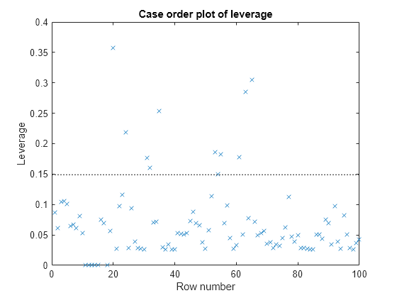
Figure contains an axes object. The axes object with title Case order plot of leverage, xlabel Row number, ylabel Leverage contains 2 objects of type line. One or more of the lines displays its values using only markers These objects represent Leverage, Reference Line.

There are a few points with high leverage. But this plot does not reveal whether the high-leverage points are outliers.

Look for points with large Cook’s distance.

plotDiagnostics(mdl,'cookd')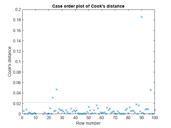

Figure contains an axes object. The axes object with title Case order plot of Cook's distance, xlabel Row number, ylabel Cook's distance contains 2 objects of type line. One or more of the lines displays its values using only markers These objects represent Cook's distance, Reference Line.

There is one point with large Cook’s distance. Identify it and remove it from the model. You can use the Data Cursor to click the outlier and identify it, or identify it programmatically:

[~,larg] = max(mdl.Diagnostics.CooksDistance);
mdl2 = fitlm(tbl,'MPG ~ Cylinders*Weight + Weight^2','Exclude',larg);

Residuals — Model Quality for Training Data

There are several residual plots to help you discover errors, outliers, or correlations in the model or data. The simplest residual plots are the default histogram plot, which shows the range of the residuals and their frequencies, and the probability plot, which shows how the distribution of the residuals compares to a normal distribution with matched variance.

Examine the residuals:

plotResiduals(mdl)

Figure contains an axes object. The axes object with title Histogram of residuals, xlabel Residuals, ylabel Probability density contains an object of type patch.

The observations above 12 are potential outliers.

plotResiduals(mdl,'probability')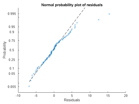

Figure contains an axes object. The axes object with title Normal probability plot of residuals, xlabel Residuals, ylabel Probability contains 2 objects of type functionline, line. One or more of the lines displays its values using only markers

The two potential outliers appear on this plot as well. Otherwise, the probability plot seems reasonably straight, meaning a reasonable fit to normally distributed residuals.

You can identify the two outliers and remove them from the data:

outl = find(mdl.Residuals.Raw > 12)

outl = 2×1

    90
    97

To remove the outliers, use the Exclude name-value pair:

mdl3 = fitlm(tbl,'MPG ~ Cylinders*Weight + Weight^2','Exclude',outl);

Examine a residuals plot of mdl2:

plotResiduals(mdl3)

Figure contains an axes object. The axes object with title Histogram of residuals, xlabel Residuals, ylabel Probability density contains an object of type patch.

The new residuals plot looks fairly symmetric, without obvious problems. However, there might be some serial correlation among the residuals. Create a new plot to see if such an effect exists.

plotResiduals(mdl3,'lagged')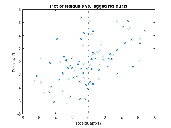

Figure contains an axes object. The axes object with title Plot of residuals vs. lagged residuals, xlabel Residual(t-1), ylabel Residual(t) contains 3 objects of type line. One or more of the lines displays its values using only markers

The scatter plot shows many more crosses in the upper-right and lower-left quadrants than in the other two quadrants, indicating positive serial correlation among the residuals.

Another potential issue is when residuals are large for large observations. See if the current model has this issue.

plotResiduals(mdl3,'fitted')

Figure contains an axes object. The axes object with title Plot of residuals vs. fitted values, xlabel Fitted values, ylabel Residuals contains 2 objects of type line. One or more of the lines displays its values using only markers

There is some tendency for larger fitted values to have larger residuals. Perhaps the model errors are proportional to the measured values.

Plots to Understand Predictor Effects

This example shows how to understand the effect each predictor has on a regression model using a variety of available plots.

Examine a slice plot of the responses. This displays the effect of each predictor separately.

plotSlice(mdl)

Figure Prediction Slice Plots contains 2 axes objects and another object of type uigridlayout. Axes object 1 contains 4 objects of type line, patch. Axes object 2 contains 3 objects of type errorbar, line.

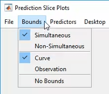
You can drag the individual predictor values, which are represented by dashed blue vertical lines. You can also choose between simultaneous and non-simultaneous confidence bounds, which are represented by dashed red curves.

Use an effects plot to show another view of the effect of predictors on the response.

plotEffects(mdl)

Figure contains an axes object. The axes object with title Main Effects Plot, xlabel Main Effect contains 4 objects of type line. One or more of the lines displays its values using only markers

This plot shows that changing Weight from about 2500 to 4732 lowers MPG by about 30 (the location of the upper blue circle). It also shows that changing the number of cylinders from 8 to 4 raises MPG by about 10 (the lower blue circle). The horizontal blue lines represent confidence intervals for these predictions. The predictions come from averaging over one predictor as the other is changed. In cases such as this, where the two predictors are correlated, be careful when interpreting the results.

Instead of viewing the effect of averaging over a predictor as the other is changed, examine the joint interaction in an interaction plot.

plotInteraction(mdl,'Weight','Cylinders')

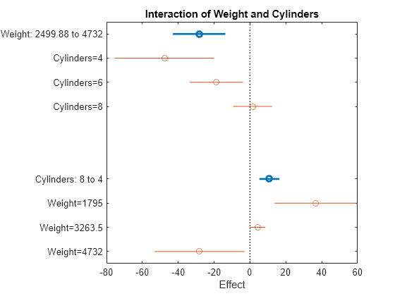
Figure contains an axes object. The axes object with title Interaction of Weight and Cylinders, xlabel Effect contains 12 objects of type line. One or more of the lines displays its values using only markers

The interaction plot shows the effect of changing one predictor with the other held fixed. In this case, the plot is much more informative. It shows, for example, that lowering the number of cylinders in a relatively light car (Weight = 1795) leads to an increase in mileage, but lowering the number of cylinders in a relatively heavy car (Weight = 4732) leads to a decrease in mileage.

For an even more detailed look at the interactions, look at an interaction plot with predictions. This plot holds one predictor fixed while varying the other, and plots the effect as a curve. Look at the interactions for various fixed numbers of cylinders.

plotInteraction(mdl,'Cylinders','Weight','predictions')

Figure contains an axes object. The axes object with title Interaction of Cylinders and Weight, xlabel Weight, ylabel Adjusted MPG contains 4 objects of type line. These objects represent Cylinders, 4, 6, 8.

Now look at the interactions with various fixed levels of weight.

plotInteraction(mdl,'Weight','Cylinders','predictions')

Figure contains an axes object. The axes object with title Interaction of Weight and Cylinders, xlabel Cylinders, ylabel Adjusted MPG contains 4 objects of type line. These objects represent Weight, 1795, 3263.5, 4732.

Plots to Understand Terms Effects

This example shows how to understand the effect of each term in a regression model using a variety of available plots.

Create an added variable plot with Weight^2 as the added variable.

plotAdded(mdl,'Weight^2')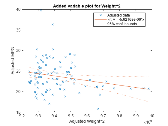

Figure contains an axes object. The axes object with title Added variable plot for Weight^2, xlabel Adjusted Weight^2, ylabel Adjusted MPG contains 3 objects of type line. One or more of the lines displays its values using only markers These objects represent Adjusted data, Fit: y = -5.62168e-06*x, 95% conf. bounds.

This plot shows the results of fitting both Weight^2 and MPG to the terms other than Weight^2. The reason to use plotAdded is to understand what additional improvement in the model you get by adding Weight^2. The coefficient of a line fit to these points is the coefficient of Weight^2 in the full model. The Weight^2 predictor is just over the edge of significance (pValue < 0.05) as you can see in the coefficients table display. You can see that in the plot as well. The confidence bounds look like they could not contain a horizontal line (constant y), so a zero-slope model is not consistent with the data.

Create an added variable plot for the model as a whole.

plotAdded(mdl)

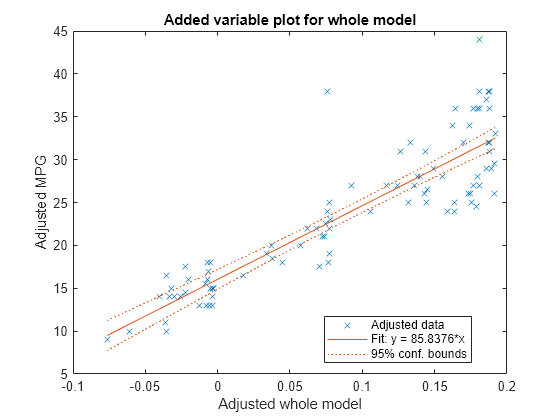
Figure contains an axes object. The axes object with title Added variable plot for whole model, xlabel Adjusted whole model, ylabel Adjusted MPG contains 3 objects of type line. One or more of the lines displays its values using only markers These objects represent Adjusted data, Fit: y = 85.8376*x, 95% conf. bounds.

The model as a whole is very significant, so the bounds don't come close to containing a horizontal line. The slope of the line is the slope of a fit to the predictors projected onto their best-fitting direction, or in other words, the norm of the coefficient vector.

Change Models

There are two ways to change a model:

step — Add or subtract terms one at a time, where step chooses the most important term to add or remove.
addTerms and removeTerms — Add or remove specified terms. Give the terms in any of the forms described in Choose a Model or Range of Models.

If you created a model using stepwiselm, then step can have an effect only if you give different upper or lower models. step does not work when you fit a model using RobustOpts.

For example, start with a linear model of mileage from the carbig data:

load carbig
tbl = table(Acceleration,Displacement,Horsepower,Weight,MPG);
mdl = fitlm(tbl,'linear','ResponseVar','MPG')

mdl = 
Linear regression model:
    MPG ~ 1 + Acceleration + Displacement + Horsepower + Weight

Estimated Coefficients:
                     Estimate         SE         tStat        pValue  
                    __________    __________    ________    __________

    (Intercept)         45.251         2.456      18.424    7.0721e-55
    Acceleration     -0.023148        0.1256     -0.1843       0.85388
    Displacement    -0.0060009     0.0067093    -0.89441       0.37166
    Horsepower       -0.043608      0.016573     -2.6312      0.008849
    Weight          -0.0052805    0.00081085     -6.5123    2.3025e-10


Number of observations: 392, Error degrees of freedom: 387
Root Mean Squared Error: 4.25
R-squared: 0.707,  Adjusted R-Squared: 0.704
F-statistic vs. constant model: 233, p-value = 9.63e-102

Try to improve the model using step for up to 10 steps:

mdl1 = step(mdl,'NSteps',10)

1. Adding Displacement:Horsepower, FStat = 87.4802, pValue = 7.05273e-19

mdl1 = 
Linear regression model:
    MPG ~ 1 + Acceleration + Weight + Displacement*Horsepower

Estimated Coefficients:
                                Estimate         SE         tStat       pValue  
                               __________    __________    _______    __________

    (Intercept)                    61.285        2.8052     21.847    1.8593e-69
    Acceleration                 -0.34401       0.11862       -2.9     0.0039445
    Displacement                -0.081198      0.010071    -8.0623    9.5014e-15
    Horsepower                   -0.24313      0.026068    -9.3265    8.6556e-19
    Weight                     -0.0014367    0.00084041    -1.7095      0.088166
    Displacement:Horsepower    0.00054236    5.7987e-05     9.3531    7.0527e-19


Number of observations: 392, Error degrees of freedom: 386
Root Mean Squared Error: 3.84
R-squared: 0.761,  Adjusted R-Squared: 0.758
F-statistic vs. constant model: 246, p-value = 1.32e-117

step stopped after just one change.

To try to simplify the model, remove the Acceleration and Weight terms from mdl1:

mdl2 = removeTerms(mdl1,'Acceleration + Weight')

mdl2 = 
Linear regression model:
    MPG ~ 1 + Displacement*Horsepower

Estimated Coefficients:
                                Estimate        SE         tStat       pValue   
                               __________    _________    _______    ___________

    (Intercept)                    53.051        1.526     34.765    3.0201e-121
    Displacement                -0.098046    0.0066817    -14.674     4.3203e-39
    Horsepower                   -0.23434     0.019593     -11.96     2.8024e-28
    Displacement:Horsepower    0.00058278    5.193e-05     11.222     1.6816e-25


Number of observations: 392, Error degrees of freedom: 388
Root Mean Squared Error: 3.94
R-squared: 0.747,  Adjusted R-Squared: 0.745
F-statistic vs. constant model: 381, p-value = 3e-115

mdl2 uses just Displacement and Horsepower, and has nearly as good a fit to the data as mdl1 in the Adjusted R-Squared metric.

Predict or Simulate Responses to New Data

Open Live Script

A LinearModel object offers three functions to predict or simulate the response to new data: predict, feval, and random.

predict

Use the predict function to predict and obtain confidence intervals on the predictions.

Load the carbig data and create a default linear model of the response MPG to the Acceleration, Displacement, Horsepower, and Weight predictors.

load carbig
X = [Acceleration,Displacement,Horsepower,Weight];
mdl = fitlm(X,MPG);

Create a three-row array of predictors from the minimal, mean, and maximal values. X contains some NaN values, so specify the 'omitnan' option for the mean function. The min and max functions omit NaN values in the calculation by default.

Xnew = [min(X);mean(X,'omitnan');max(X)];

Find the predicted model responses and confidence intervals on the predictions.

[NewMPG, NewMPGCI] = predict(mdl,Xnew)

NewMPG = 3×1

   34.1345
   23.4078
    4.7751

NewMPGCI = 3×2

   31.6115   36.6575
   22.9859   23.8298
    0.6134    8.9367

The confidence bound on the mean response is narrower than those for the minimum or maximum responses.

feval

Use the feval function to predict responses. When you create a model from a table or dataset array, feval is often more convenient than predict for predicting responses. When you have new predictor data, you can pass it to feval without creating a table or matrix. However, feval does not provide confidence bounds.

Load the carbig data set and create a default linear model of the response MPG to the predictors Acceleration, Displacement, Horsepower, and Weight.

load carbig
tbl = table(Acceleration,Displacement,Horsepower,Weight,MPG);
mdl = fitlm(tbl,'linear','ResponseVar','MPG');

Predict the model response for the mean values of the predictors.

NewMPG = feval(mdl,mean(Acceleration,'omitnan'),mean(Displacement,'omitnan'),mean(Horsepower,'omitnan'),mean(Weight,'omitnan'))

NewMPG = 
23.4078

random

Use the random function to simulate responses. The random function simulates new random response values, equal to the mean prediction plus a random disturbance with the same variance as the training data.

Load the carbig data and create a default linear model of the response MPG to the Acceleration, Displacement, Horsepower, and Weight predictors.

load carbig
X = [Acceleration,Displacement,Horsepower,Weight];
mdl = fitlm(X,MPG);

Create a three-row array of predictors from the minimal, mean, and maximal values.

Xnew = [min(X);mean(X,'omitnan');max(X)];

Generate new predicted model responses including some randomness.

rng('default') % for reproducibility
NewMPG = random(mdl,Xnew)

NewMPG = 3×1

   36.4178
   31.1958
   -4.8176

Because a negative value of MPG does not seem sensible, try predicting two more times.

NewMPG = random(mdl,Xnew)

NewMPG = 3×1

   37.7959
   24.7615
   -0.7783

NewMPG = random(mdl,Xnew)

NewMPG = 3×1

   32.2931
   24.8628
   19.9715

Clearly, the predictions for the third (maximal) row of Xnew are not reliable.

Share Fitted Models

Open Live Script

Suppose you have a linear regression model, such as mdl from the following commands.

load carbig
tbl = table(Acceleration,Displacement,Horsepower,Weight,MPG);
mdl = fitlm(tbl,'linear','ResponseVar','MPG');

To share the model with other people, you can:

Provide the model display.

mdl

mdl = 
Linear regression model:
    MPG ~ 1 + Acceleration + Displacement + Horsepower + Weight

Estimated Coefficients:
                     Estimate         SE         tStat        pValue  
                    __________    __________    ________    __________

    (Intercept)         45.251         2.456      18.424    7.0721e-55
    Acceleration     -0.023148        0.1256     -0.1843       0.85388
    Displacement    -0.0060009     0.0067093    -0.89441       0.37166
    Horsepower       -0.043608      0.016573     -2.6312      0.008849
    Weight          -0.0052805    0.00081085     -6.5123    2.3025e-10


Number of observations: 392, Error degrees of freedom: 387
Root Mean Squared Error: 4.25
R-squared: 0.707,  Adjusted R-Squared: 0.704
F-statistic vs. constant model: 233, p-value = 9.63e-102

Provide the model definition and coefficients.

mdl.Formula

ans = 
MPG ~ 1 + Acceleration + Displacement + Horsepower + Weight

mdl.CoefficientNames

ans = 1x5 cell
    {'(Intercept)'}    {'Acceleration'}    {'Displacement'}    {'Horsepower'}    {'Weight'}

mdl.Coefficients.Estimate

ans = 5×1

   45.2511
   -0.0231
   -0.0060
   -0.0436
   -0.0053