Visualize and Apply Image Embeddings for Classification
R2026bThis example shows how to use image embeddings from the CLIP (Contrastive Language-Image Pre-training) [1] model to classify images without training a custom model. CLIP learns a shared embedding space for images and text. This enables you to classify images by using text descriptions alone, compare images directly by their embeddings, and detect anomalies by contrasting normal and abnormal text prompts.
In this example, you:
Visualize high-dimensional image and text embeddings in a low-dimensional space by using dimensionality reduction techniques.
Classify images using text-prompted and image exemplar methods.
Download VisA Data Set
This example uses a subset of the VisA (Visual Anomaly) data set [2], which contains industrial inspection images of objects across multiple categories. Each category has normal images and images with defects.
Download the data set and unzip the contents into a temporary folder.
dataDir = fullfile(tempdir,"VisA");
downloadVisAData(dataDir)
Prepare Data Set
Select six classes from the VisA data set and use 50 images from each class. Consider decreasing the number of images per class if no GPU is available, because generating the image embeddings on CPU is time-consuming.
samplesPerClass =  50
50samplesPerClass = 50
classNames = ["candle","capsules","cashew","chewinggum","macaroni1","pcb2"];
classDescriptions = ["candle","pills","cashew","chewing gum","macaroni pasta", ...
    "printed circuit board"];

imds = imageDatastore(fullfile(dataDir,"VisA",classNames,"test","good"));
Assign class labels extracted from the folder structure by using the helperExtractClassLabels helper function, included in the supporting project file attached to this example.
classLabels = helperExtractClassLabels(imds.Files);
imds.Labels = classLabels;
Subsample the data set by using the subsampleDatastore helper function, included in the supporting project file attached to this example. Set the random number generator state to ensure deterministic sampling.
rng("default")
imds = subsampleDatastore(imds,samplesPerClass);
Re-extract class labels after subsampling.
classLabels = helperExtractClassLabels(imds.Files);
Rename the folder-based class labels to human-readable descriptions. Using natural language names such as "pills" instead of "capsules" better matches CLIP training data and improves text prompt accuracy.
classLabels = renamecats(classLabels,classNames,classDescriptions);
imds.Labels = renamecats(imds.Labels,classNames,classDescriptions);
classNames = classDescriptions;
Preview Image Data
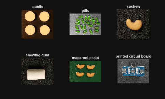
Display one sample image from each class by using the helperPreviewClasses helper function, included in the supporting project file attached to this example.
helperPreviewClasses(classNames,classLabels,imds);
Load CLIP Network
Create a pretrained CLIP network by using the clipNetwork object. The CLIP model encodes both images and text into a shared embedding space, where semantically similar content maps to nearby points.
Select a CLIP backbone. Larger backbones have more parameters, which produces more discriminative embeddings but requires more computation time.
Backbone | Approximate Parameter Count |
| 428 million |
| 150 million |
| 102 million |
backbone =  "resnet50";
clip = clipNetwork(backbone);
"resnet50";
clip = clipNetwork(backbone);Extract Image Embeddings
Extract a fixed-length embedding vector for each image by using the extractImageEmbeddings function. These embeddings capture the visual content of each image in a numerically comparable form. The function automatically uses a GPU if one is available, which significantly reduces computation time. Processing image data on a GPU requires a supported GPU device and Parallel Computing Toolbox™. This operation might take several minutes on CPU.
imageEmbeddingsRaw = extractImageEmbeddings(clip,imds);
Display the size of imageEmbeddingsRaw to verify the embedding dimensions.
disp(size(imageEmbeddingsRaw));
768 300
The orientation of CLIP embeddings matters more than their location, because CLIP was trained with cosine similarity. Normalize the embeddings to unit length to improve visualization after dimensionality reduction while preserving directional information.
imageEmbeddings = normalize(imageEmbeddingsRaw,"norm");Visualize Embeddings
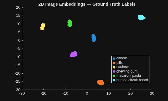
To visualize the high-dimensional embeddings, reduce them to 2 or 3 dimensions to determine how similar images cluster together in the embedding space.
When you compress high-dimensional embeddings into a low-dimensional space, you discard some information. Aim to preserve relative distances between the embeddings while discarding noise.
Specify the dimensionality reduction method by using one of these functions:
tsne(Statistics and Machine Learning Toolbox) — t-distributed stochastic neighbor embedding (t-SNE). Preserves local neighborhood structure, making it effective for revealing tight clusters.pca(Statistics and Machine Learning Toolbox) — Principal component analysis. A linear method that preserves global variance and runs faster than nonlinear alternatives.umap(Statistics and Machine Learning Toolbox) — Uniform Manifold Approximation and Projection (UMAP). Balances local and global structure, often producing well-separated clusters with meaningful inter-cluster distances.
useMethod =  "umap";
Perform the dimensionality reduction by using the helperReduceDims helper function, included in the supporting project file attached to this example. For the t-SNE and UMAP methods, this helper sets the Distance name-value argument to "cosine" because CLIP was trained by using cosine similarity.
embeddingsMatrix = imageEmbeddings';
reduction2D = helperReduceDims(embeddingsMatrix,useMethod,2);
reduction3D = helperReduceDims(embeddingsMatrix,useMethod,3);
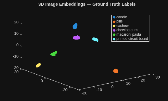
Plot the embeddings colored by ground truth class label in 2-D or 3-D, depending on the dimensionality of the reduced data, by using the helperScatterND helper function, included in the supporting project file attached to this example. Similar images cluster together because the CLIP encoder maps them to nearby points.
figure
hold on
classes = categories(classLabels);
colors = lines(numel(classes));

for c = 1:numel(classes)
    idx = classLabels == classes(c);
    helperScatterND(reduction2D(idx,:),30,colors(c,:),"o", ...
        "filled",DisplayName=string(classes(c)));
end
hold off

legend(Location="best")
title("2D Image Embeddings — Ground Truth Labels")
Now plot in three dimensions.
figure
hold on
classes = categories(classLabels);
colors = lines(numel(classes));

for c = 1:numel(classes)
    idx = classLabels == classes(c);
    helperScatterND(reduction3D(idx,:),30,colors(c,:),"o", ...
        "filled",DisplayName=string(classes(c)));
end
hold off
legend(Location="best")
title("3D Image Embeddings — Ground Truth Labels")
Classify Images Using Embeddings
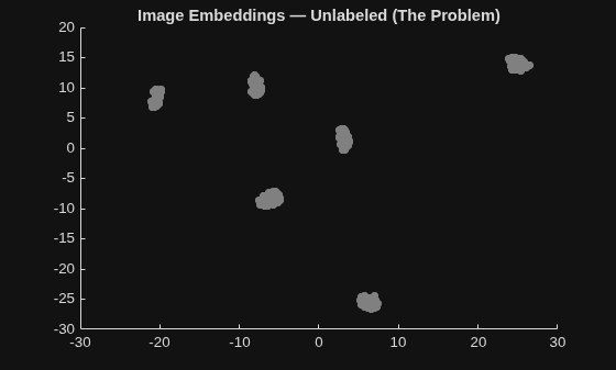
Consider a realistic scenario: you have collected a data set of images but have not labeled them. You have only a list of images with no metadata. One of the challenges in processing the images is to classify them into categories. Using image embeddings for this task saves time that you would otherwise spend on manual annotation and labeling.
Plot the same embeddings without color to illustrate this challenge by using the helperScatterND helper function.
figure
helperScatterND(reduction2D,30,[0.5 0.5 0.5],"o","filled")
title("Image Embeddings — Unlabeled (The Problem)")
Classify Images Using Text Prompts
Because CLIP maps images and text into the same embedding space, you can classify images by comparing them to text descriptions of each class, without requiring any training images as reference. The text descriptions are open-vocabulary and are not limited to a fixed set of descriptions.
To classify images by using text prompts:
Encode each class name as a text embedding (for example, "A photo of a candle").
Compute cosine similarity between each image embedding and each text embedding.
Assign each image to the class whose text embedding is most similar.
The embedding model might rank a particular image higher for one phrasing of a text prompt than for a synonymous phrasing. For example, an image might score higher with the prompt "an image of a cat" than with "a photo of a cat". Prompt ensembling reduces this sensitivity. When you use ensembled prompts, the classify function averages embeddings from multiple prompt templates per class (for example, "A photo of a [class]", "An image of a [class]", and so on) for more robust classification. With a single prompt, the function uses only "A photo of [class]".
Extract the text embeddings from the prompts for visualization in the next section. If you use simple prompts, compute similarity scores in single precision by using the pdist2 (Statistics and Machine Learning Toolbox) function with cosine distance.
ensembleTextPrompts =true; simplePrompt = "A photo of " + classNames; textEmbForVisualization = extractTextEmbeddings(clip,simplePrompt); textEmbForVisualization = normalize(textEmbForVisualization,"norm"); if ensembleTextPrompts [~,textSimScores] = classify(clip,imds,classNames); else textSimScores = 1 - pdist2(single(imageEmbeddings'),single(textEmbForVisualization'),"cosine"); end
Display the size of textSimScores. The text cosine similarity scores include one row per image. Each column in that row contains the cosine similarity between the image and one of the classes.
disp(size(textSimScores));
300 6
Predict image classes by assigning each image to the class with the maximum cosine similarity.
[~,predictedIdxText] = max(textSimScores,[],2);
predictedLabelsText = classNames(predictedIdxText)';
Visualize Text and Image Embeddings in Shared Space
Visualize the text prompt embeddings alongside the image embeddings in the shared space. The star markers indicate where each text prompt lands relative to the image clusters. This visualization uses only the simple prompt embeddings, not the ensembled prompt embeddings.
To preserve relative locations, reduce both the text and image embeddings together. Specify a combined matrix as input to the helperReduceDims helper function.
allEmbeddings = [embeddingsMatrix; textEmbForVisualization'];
reductionWithText2D = helperReduceDims(allEmbeddings,useMethod,2);

nImages = size(embeddingsMatrix,1);
reductionImages2D = reductionWithText2D(1:nImages,:);
reductionText2D = reductionWithText2D(nImages+1:end,:);
Plot the image embeddings as dots by using the helperScatterND helper function.
figure
hold on
for c = 1:numel(classes)
    idx = classLabels == classes(c);
    helperScatterND(reductionImages2D(idx,:),30,colors(c,:),"o", ...
        "filled",HandleVisibility="off")
end
Visualize the text embeddings as stars.
for c = 1:numel(classNames)
    colorIdx = find(classes == classNames(c));
    helperScatterND(reductionText2D(c,:),300,colors(colorIdx,:),"pentagram", ...
        "filled",DisplayName=simplePrompt(c),MarkerEdgeColor='w');
end
hold off
legend(Location="bestoutside")
title("2D Image + Text Embeddings in Shared Space")
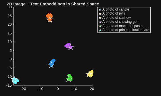
Now plot in three dimensions.
reductionWithText3D = helperReduceDims(allEmbeddings,useMethod,3);
reductionImages3D = reductionWithText3D(1:nImages,:);
reductionText3D = reductionWithText3D(nImages+1:end,:);

figure
hold on
for c = 1:numel(classes)
    idx = classLabels == classes(c);
    helperScatterND(reductionImages3D(idx,:),30,colors(c,:),"o", ...
        "filled",HandleVisibility="off")
end

for c = 1:numel(classNames)
    colorIdx = find(classes == classNames(c));
    helperScatterND(reductionText3D(c,:),300,colors(colorIdx,:),"pentagram", ...
        "filled",DisplayName=simplePrompt(c),MarkerEdgeColor='w');
end
hold off
legend(Location="bestoutside")
title("3D Image + Text Embeddings in Shared Space")
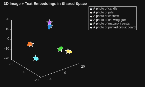
Evaluate Text Prompt Classification Accuracy
Evaluate classification accuracy by using a confusion matrix. Because CLIP was trained on internet-scale image-text pairs, it can often distinguish visually distinct categories with no task-specific training.
figure
trueLabels = string(classLabels);
confusionchart(trueLabels,predictedLabelsText)
title("Confusion Matrix — Text-Prompted Classification")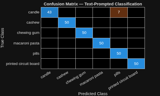
The model misclassifies only 7 of 250 images.
Examine a misclassification to understand where text-prompted classification struggles. The bar chart shows the softmax of similarity scores for all classes, computed by using the softmax (Deep Learning Toolbox) function. Ideally, the true class (green) dominates.
misclassIdxText = find(predictedLabelsText ~= trueLabels,1);
if ~isempty(misclassIdxText)
    figure
    tiledlayout(1,2)
    nexttile
    imshow(readimage(imds,misclassIdxText))
    title("Misclassified Image (True: " + string(classLabels(misclassIdxText)) + ")")
    nexttile
    barColors = repmat([0.4 0.4 0.8],numel(classNames),1);
    trueClassIdx = find(classNames == string(classLabels(misclassIdxText)));
    barColors(trueClassIdx,:) = [0 0.7 0];
    classProbabilities = softmax(dlarray(textSimScores(misclassIdxText,:)),DataFormat='BC');
    b = bar(extractdata(classProbabilities));
    b.FaceColor = "flat";
    b.CData = barColors;
    set(gca,XTickLabel=classNames)
    ylabel("Probability")
    title("Softmax of Similarity Scores")
end
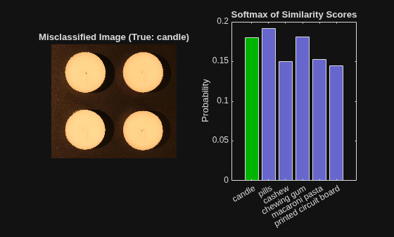
The true class ranks as the third most likely class for this image. The top two predicted classes, pills and chewing gum, are also plausible given the shape and number of candles in the image.
Classify Images by Using Image Exemplars
Instead of text, you can classify images by comparing them to a representative image from each class. This is useful when you have example images but cannot easily describe the categories in words.
To classify images by using exemplars:
Select one exemplar image per class.
Compute cosine similarity between each image embedding and each exemplar embedding.
Assign each image to the class whose exemplar is most similar.
Select one exemplar image per class. For this example, selecting exemplars is automated by using the VisA class labels. In a real-world scenario, you typically select exemplars manually because class labels are not available.
exemplarEmbeddings = zeros(size(imageEmbeddings,1),numel(classes));
for c = 1:numel(classes)
    idx = find(classLabels == classes(c),1);
    exemplarEmbeddings(:,c) = imageEmbeddings(:,idx);
end
Compute cosine similarity between each image embedding and each exemplar embedding by using the pdist2 (Statistics and Machine Learning Toolbox) function with cosine distance.
simScores = 1 - pdist2(single(imageEmbeddings'),single(exemplarEmbeddings'),"cosine");Assign each image to the class whose exemplar is most similar.
[~,predictedIdxImage] = max(simScores,[],2);
predictedLabelsImage = string(classes(predictedIdxImage));
Evaluate Image Exemplar Classification Accuracy
Evaluate classification accuracy by using a confusion matrix.
figure
confusionchart(trueLabels,predictedLabelsImage)
title("Confusion Matrix — Image-Prompted Classification")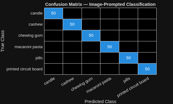
The image-prompted classification achieves 100% accuracy.
In this example, you classified images by using two different methods, text prompts and exemplar images, both without any model training. This is possible because CLIP was trained on internet-scale image-text data, giving it broad visual and semantic understanding. The classification is open-vocabulary and zero-shot: you can specify arbitrary class names without retraining or fine-tuning.
Outlook
Extend this procedure to other embedding models, such as DINOv2, for fine-grained visual similarity tasks. For data sets with unknown class labels, apply unsupervised clustering methods such as k-means or spectral clustering directly on the embedding vectors to discover groupings. Beyond classification, embeddings enable other capabilities such as image retrieval and anomaly detection.
Define Helper Functions
helperExtractClassLabels
Use this function to extract the class name from each file path based on the VisA data set folder structure. The VisA data set stores files in the path format VisA/className/test/good/ABCD.jpg.
function classLabels = helperExtractClassLabels(filePaths)
    classLabels = strings(numel(filePaths),1);
    for i = 1:numel(filePaths)
        parts = split(filePaths{i},filesep);
        classLabels(i) = parts{end-3};
    end
    classLabels = categorical(classLabels);
end
helperPreviewClasses
Use this function to display a montage with one image per class from the provided datastore.
function helperPreviewClasses(classNames,classLabels,imds)
    figure
    tiledlayout
    for c = 1:numel(classNames)
        idx = find(classLabels == classNames(c),1);
        nexttile
        imshow(readimage(imds,idx))
        title(classNames(c))
    end
end
helperReduceDims
Use this function to reduce the dimensionality of embedding data by using the specified method and number of output dimensions. To tune hyperparameters, see tsne (Statistics and Machine Learning Toolbox), pca (Statistics and Machine Learning Toolbox), or umap (Statistics and Machine Learning Toolbox).
function reduction = helperReduceDims(data,method,numDims)
    switch method
        case "tsne"
            reduction = tsne(data,NumDimensions=numDims,Distance="cosine");
        case "pca"
            [~,reduction] = pca(data,NumComponents=numDims);
        case "umap"
            reduction = umap(data,NumDimensions=numDims,Distance="cosine", ...
                Reproducible=true,EmbeddingDensity=0.5);
    end
end
helperScatterND
Use this function to create a scatter plot in either 2-D or 3-D depending on the number of columns in the input data.
function helperScatterND(pts,sz,color,varargin)
    if size(pts,2) == 3
        scatter3(pts(:,1),pts(:,2),pts(:,3),sz,color,varargin{:});
        view(3);
    else
        scatter(pts(:,1),pts(:,2),sz,color,varargin{:});
    end
end
References
[1] Radford, Alec, Jong Wook Kim, Chris Hallacy, Aditya Ramesh, Gabriel Goh, Sandhini Agarwal, Girish Sastry, Amanda Askell, Pamela Mishkin, Jack Clark, Gretchen Krueger, and Ilya Sutskever. "Learning Transferable Visual Models from Natural Language Supervision." In Proceedings of the 38th International Conference on Machine Learning, 8748–8763. PMLR, 2021. https://doi.org/10.48550/arXiv.2103.00020.
[2] Zou, Yang, Jongheon Jeong, Latha Pemula, Dongqing Zhang, and Onkar Dabeer. "SPot-the-Difference Self-Supervised Pre-Training for Anomaly Detection and Segmentation." arXiv preprint arXiv:2207.14315 (2022). https://doi.org/10.48550/arXiv.2207.14315.
See Also
clipNetwork | extractImageEmbeddings | classify

