Acoustic Scene Recognition Using Late Fusion

This example uses:

This example shows how to create a multi-model late fusion system for acoustic scene recognition. The example trains a convolutional neural network (CNN) using mel spectrograms and an ensemble classifier using wavelet scattering. The example uses the TUT dataset for training and evaluation [1].

Introduction

Acoustic scene classification (ASC) is the task of classifying environments from the sounds they produce. ASC is a generic classification problem that is foundational for context awareness in devices, robots, and many other applications [1]. Early attempts at ASC used mel-frequency cepstral coefficients (mfcc (Audio Toolbox)) and Gaussian mixture models (GMMs) to describe their statistical distribution. Other popular features used for ASC include zero crossing rate, spectral centroid (spectralCentroid (Audio Toolbox)), spectral rolloff (spectralRolloffPoint (Audio Toolbox)), spectral flux (spectralFlux (Audio Toolbox) ), and linear prediction coefficients (lpc (Signal Processing Toolbox)) [5]. Hidden Markov models (HMMs) were trained to describe the temporal evolution of the GMMs. More recently, the best performing systems have used deep learning, usually CNNs, and a fusion of multiple models. The most popular feature for top-ranked systems in the DCASE 2017 contest was the mel spectrogram (melSpectrogram (Audio Toolbox)). The top-ranked systems in the challenge used late fusion and data augmentation to help their systems generalize.

To illustrate a simple approach that produces reasonable results, this example trains a CNN using mel spectrograms and an ensemble classifier using wavelet scattering. The CNN and ensemble classifier produce roughly equivalent overall accuracy, but perform better at distinguishing different acoustic scenes. To increase overall accuracy, you merge the CNN and ensemble classifier results using late fusion.

Load Acoustic Scene Recognition Data Set

To run the example, you must first download the data set [1]. The full data set is approximately 15.5 GB. Depending on your machine and internet connection, downloading the data can take about 4 hours.

downloadFolder = tempdir;
dataset = fullfile(downloadFolder,"TUT-acoustic-scenes-2017");

if ~datasetExists(dataset)
    disp("Downloading TUT-acoustic-scenes-2017 (15.5 GB) ...")
    HelperDownload_TUT_acoustic_scenes_2017(dataset);
end

Read in the development set metadata as a table. Name the table variables FileName, AcousticScene, and SpecificLocation.

trainMetaData = readtable(fullfile(dataset,"TUT-acoustic-scenes-2017-development","meta"), ...
    Delimiter={'\t'}, ...
    ReadVariableNames=false);
trainMetaData.Properties.VariableNames = ["FileName","AcousticScene","SpecificLocation"];
head(trainMetaData)

             FileName             AcousticScene    SpecificLocation
    __________________________    _____________    ________________

    {'audio/b020_90_100.wav' }      {'beach'}          {'b020'}    
    {'audio/b020_110_120.wav'}      {'beach'}          {'b020'}    
    {'audio/b020_100_110.wav'}      {'beach'}          {'b020'}    
    {'audio/b020_40_50.wav'  }      {'beach'}          {'b020'}    
    {'audio/b020_50_60.wav'  }      {'beach'}          {'b020'}    
    {'audio/b020_30_40.wav'  }      {'beach'}          {'b020'}    
    {'audio/b020_160_170.wav'}      {'beach'}          {'b020'}    
    {'audio/b020_170_180.wav'}      {'beach'}          {'b020'}

testMetaData = readtable(fullfile(dataset,"TUT-acoustic-scenes-2017-evaluation","meta"), ...
    Delimiter={'\t'}, ...
    ReadVariableNames=false);
testMetaData.Properties.VariableNames = ["FileName","AcousticScene","SpecificLocation"];
head(testMetaData)

         FileName         AcousticScene    SpecificLocation
    __________________    _____________    ________________

    {'audio/1245.wav'}      {'beach'}          {'b174'}    
    {'audio/1456.wav'}      {'beach'}          {'b174'}    
    {'audio/1318.wav'}      {'beach'}          {'b174'}    
    {'audio/967.wav' }      {'beach'}          {'b174'}    
    {'audio/203.wav' }      {'beach'}          {'b174'}    
    {'audio/777.wav' }      {'beach'}          {'b174'}    
    {'audio/231.wav' }      {'beach'}          {'b174'}    
    {'audio/768.wav' }      {'beach'}          {'b174'}

Note that the specific recording locations in the test set do not intersect with the specific recording locations in the development set. This makes it easier to validate that the trained models can generalize to real-world scenarios.

sharedRecordingLocations = intersect(testMetaData.SpecificLocation,trainMetaData.SpecificLocation);
disp("Number of specific recording locations in both train and test sets = " + numel(sharedRecordingLocations))

Number of specific recording locations in both train and test sets = 0

The first variable of the metadata tables contains the file names. Concatenate the file names with the file paths.

trainFilePaths = fullfile(dataset,"TUT-acoustic-scenes-2017-development",trainMetaData.FileName);

testFilePaths = fullfile(dataset,"TUT-acoustic-scenes-2017-evaluation",testMetaData.FileName);

There may be files listed in the metadata that are not present in the data set. Remove the file paths and acoustic scene labels that correspond to the missing files.

ads = audioDatastore(dataset,IncludeSubfolders=true);
allFiles = ads.Files;

trainIdxToRemove = ~ismember(trainFilePaths,allFiles);
trainFilePaths(trainIdxToRemove) = [];
trainLabels = categorical(trainMetaData.AcousticScene);
trainLabels(trainIdxToRemove) = [];

testIdxToRemove = ~ismember(testFilePaths,allFiles);
testFilePaths(testIdxToRemove) = [];
testLabels = categorical(testMetaData.AcousticScene);
testLabels(testIdxToRemove) = [];

Create audio datastores for the train and test sets. Set the Labels property of the audioDatastore (Audio Toolbox) to the acoustic scene. Call countEachLabel (Audio Toolbox) to verify an even distribution of labels in both the train and test sets.

adsTrain = audioDatastore(trainFilePaths, ...
    Labels=trainLabels, ...
    IncludeSubfolders=true);
display(countEachLabel(adsTrain))

  15×2 table

         Label          Count
    ________________    _____

    beach                312 
    bus                  312 
    cafe/restaurant      312 
    car                  312 
    city_center          312 
    forest_path          312 
    grocery_store        312 
    home                 312 
    library              312 
    metro_station        312 
    office               312 
    park                 312 
    residential_area     312 
    train                312 
    tram                 312

adsTest = audioDatastore(testFilePaths, ...
    Labels=testLabels, ...
    IncludeSubfolders=true);
display(countEachLabel(adsTest))

  15×2 table

         Label          Count
    ________________    _____

    beach                108 
    bus                  108 
    cafe/restaurant      108 
    car                  108 
    city_center          108 
    forest_path          108 
    grocery_store        108 
    home                 108 
    library              108 
    metro_station        108 
    office               108 
    park                 108 
    residential_area     108 
    train                108 
    tram                 108

You can reduce the data set used in this example to speed up the run time at the cost of performance. In general, reducing the data set is a good practice for development and debugging. Set speedupExample to true to reduce the data set.

speedupExample = false;
if speedupExample
    adsTrain = splitEachLabel(adsTrain,20);
    adsTest = splitEachLabel(adsTest,10);
end
trainLabels = adsTrain.Labels;
testLabels = adsTest.Labels;

Call read (Audio Toolbox) to get the data and sample rate of a file from the train set. Audio in the database has consistent sample rate and duration. Normalize the audio and listen to it. Display the corresponding label.

[data,adsInfo] = read(adsTrain);
data = data./max(data,[],"all");

fs = adsInfo.SampleRate;
sound(data,fs)

disp("Acoustic scene = " + string(adsTrain.Labels(1)))

Acoustic scene = beach

Call reset (Audio Toolbox) to return the datastore to its initial condition.

reset(adsTrain)

Feature Extraction for CNN

Each audio clip in the dataset consists of 10 seconds of stereo (left-right) audio. The feature extraction pipeline and the CNN architecture in this example are based on [3]. Hyperparameters for the feature extraction, the CNN architecture, and the training options were modified from the original paper using a systematic hyperparameter optimization workflow.

First, convert the audio to mid-side encoding. [3] suggests that mid-side encoded data provides better spatial information that the CNN can use to identify moving sources (such as a train moving across an acoustic scene).

dataMidSide = [sum(data,2),data(:,1)-data(:,2)];

Divide the signal into one-second segments with overlap. The final system uses a probability-weighted average on the one-second segments to predict the scene for each 10-second audio clip in the test set. Dividing the audio clips into one-second segments makes the network easier to train and helps prevent overfitting to specific acoustic events in the training set. The overlap helps to ensure all combinations of features relative to one another are captured by the training data. It also provides the system with additional data that can be mixed uniquely during augmentation.

segmentLength = 1;
segmentOverlap = 0.5;

[dataBufferedMid,~] = buffer(dataMidSide(:,1),round(segmentLength*fs),round(segmentOverlap*fs),"nodelay");
[dataBufferedSide,~] = buffer(dataMidSide(:,2),round(segmentLength*fs),round(segmentOverlap*fs),"nodelay");
dataBuffered = zeros(size(dataBufferedMid,1),size(dataBufferedMid,2)+size(dataBufferedSide,2));
dataBuffered(:,1:2:end) = dataBufferedMid;
dataBuffered(:,2:2:end) = dataBufferedSide;

Use melSpectrogram (Audio Toolbox) to transform the data into a compact frequency-domain representation. Define parameters for the mel spectrogram as suggested by [3].

windowLength = 2048;
samplesPerHop = 1024;
samplesOverlap = windowLength - samplesPerHop;
fftLength = 2*windowLength;
numBands = 128;

melSpectrogram operates along channels independently. To optimize processing time, call melSpectrogram with the entire buffered signal.

spec = melSpectrogram(dataBuffered,fs, ...
    Window=hamming(windowLength,"periodic"), ...
    OverlapLength=samplesOverlap, ...
    FFTLength=fftLength, ...
    NumBands=numBands, ...
    ApplyLog=true);

Reshape the array to dimensions (Number of bands)-by-(Number of hops)-by-(Number of channels)-by-(Number of segments). When you feed an image into a neural network, the first two dimensions are the height and width of the image, the third dimension is the channels, and the fourth dimension separates the individual images.

X = reshape(spec,size(spec,1),size(spec,2),size(data,2),[]);

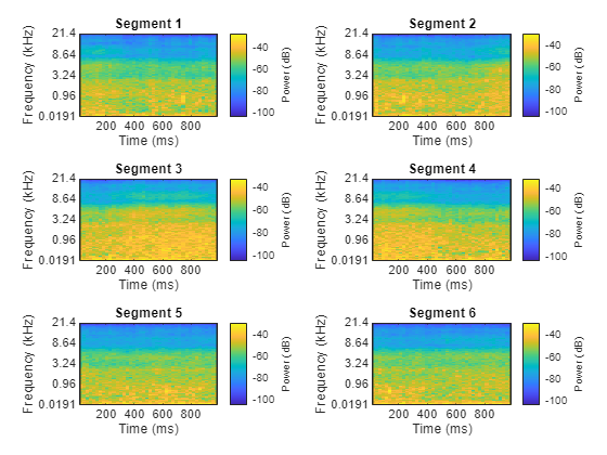
Call melSpectrogram without output arguments to plot the mel spectrogram of the mid channel for the first six of the one-second increments.

tiledlayout(3,2)
for channel = 1:2:11
    nexttile
    melSpectrogram(dataBuffered(:,channel),fs, ...
        Window=hamming(windowLength,"periodic"), ...
        OverlapLength=samplesOverlap, ...
        FFTLength=fftLength, ...
        NumBands=numBands, ...
        ApplyLog=true);
    title("Segment " + ceil(channel/2))
end

The helper function HelperSegmentedMelSpectrograms performs the feature extraction steps outlined above.

To apply the feature extraction steps to all files in the datastores, create transform datastores and specify the HelperSegmentedMelSpectrograms function as the transform. To speed up subsequent processing, use readall to read all of the files and place the extracted features in memory. Transform datastores can leverage parallel pools to speed up file reading and preprocessing if you have Parallel Computing Toolbox™.

tdsTrain = transform(adsTrain,@(x){HelperSegmentedMelSpectrograms(x,fs, ...
    SegmentLength=segmentLength, ...
    SegmentOverlap=segmentOverlap, ...
    WindowLength=windowLength, ...
    HopLength=samplesPerHop, ...
    NumBands=numBands, ...
    FFTLength=fftLength)});
xTrain = readall(tdsTrain,UseParallel=canUseParallelPool);

Starting parallel pool (parpool) using the 'local' profile ...
16-Nov-2023 12:40:45: Job Queued. Waiting for parallel pool job with ID 1 to start ...
16-Nov-2023 12:41:46: Job Queued. Waiting for parallel pool job with ID 1 to start ...
Connected to parallel pool with 6 workers.

xTrain = cat(4,xTrain{:});

tdsTest = transform(adsTest,@(x){HelperSegmentedMelSpectrograms(x,fs, ...
    SegmentLength=segmentLength, ...
    SegmentOverlap=segmentOverlap, ...
    WindowLength=windowLength, ...
    HopLength=samplesPerHop, ...
    NumBands=numBands, ...
    FFTLength=fftLength)});
xTest = readall(tdsTest,UseParallel=canUseParallelPool);
xTest = cat(4,xTest{:});

Replicate the labels of the training and test sets so that they are in one-to-one correspondence with the segments.

numSegmentsPer10seconds = size(dataBuffered,2)/2;
yTrain = repmat(trainLabels,1,numSegmentsPer10seconds)';
yTrain = yTrain(:);
yTest = repmat(testLabels,1,numSegmentsPer10seconds)';
yTest = yTest(:);

Data Augmentation for CNN

The DCASE 2017 dataset contains a relatively small number of acoustic recordings for the task, and the development set and evaluation set were recorded at different specific locations. As a result, it is easy to overfit to the data during training. One popular method to reduce overfitting is mixup. In mixup, you augment your dataset by mixing the features of two different classes. When you mix the features, you mix the labels in equal proportion. That is:

$\begin{array}{l} x_{}^{\sim} = λ x_{i} + (1 - λ) x_{j} \\ y_{}^{\sim} = λ y_{i} + (1 - λ) y_{j} \end{array}$

Mixup was reformulated by [2] as labels drawn from a probability distribution instead of mixed labels. The implementation of mixup in this example is a simplified version of mixup: each spectrogram is mixed with a spectrogram of a different label with lambda set to 0.5. The original and mixed datasets are combined for training.

xTrainExtra = xTrain;
yTrainExtra = yTrain;
lambda = 0.5;
for ii = 1:size(xTrain,4)
    
    % Find all available spectrograms with different labels.
    availableSpectrograms = find(yTrain~=yTrain(ii));
    
    % Randomly choose one of the available spectrograms with a different label.
    numAvailableSpectrograms = numel(availableSpectrograms);
    idx = randi([1,numAvailableSpectrograms]);
    
    % Mix.
    xTrainExtra(:,:,:,ii) = lambda*xTrain(:,:,:,ii) + (1-lambda)*xTrain(:,:,:,availableSpectrograms(idx));
    
    % Specify the label as randomly set by lambda.
    if rand > lambda
        yTrainExtra(ii) = yTrain(availableSpectrograms(idx));
    end
end
xTrain = cat(4,xTrain,xTrainExtra);
yTrain = [yTrain;yTrainExtra];

Call summary to display the distribution of labels for the augmented training set.

summary(yTrain)

     beach                 11769 
     bus                   11904 
     cafe/restaurant       11873 
     car                   11820 
     city_center           11886 
     forest_path           11936 
     grocery_store         11914 
     home                  11923 
     library               11817 
     metro_station         11804 
     office                11922 
     park                  11871 
     residential_area      11704 
     train                 11773 
     tram                  11924

Define and Train CNN

Define the CNN architecture. This architecture is based on [1] and modified through trial and error. See List of Deep Learning Layers (Deep Learning Toolbox) to learn more about deep learning layers available in MATLAB®.

imgSize = [size(xTrain,1),size(xTrain,2),size(xTrain,3)];
numF = 32;
layers = [ ...
    imageInputLayer(imgSize)
    
    batchNormalizationLayer
    
    convolution2dLayer(3,numF,Padding="same")
    batchNormalizationLayer
    reluLayer
    convolution2dLayer(3,numF,Padding="same")
    batchNormalizationLayer
    reluLayer 
    
    maxPooling2dLayer(3,Stride=2,Padding="same")

    convolution2dLayer(3,2*numF,Padding="same")
    batchNormalizationLayer
    reluLayer
    convolution2dLayer(3,2*numF,Padding="same")
    batchNormalizationLayer
    reluLayer
    
    maxPooling2dLayer(3,Stride=2,Padding="same")
    
    convolution2dLayer(3,4*numF,Padding="same")
    batchNormalizationLayer
    reluLayer
    convolution2dLayer(3,4*numF,Padding="same")
    batchNormalizationLayer
    reluLayer
    
    maxPooling2dLayer(3,Stride=2,Padding="same")
    
    convolution2dLayer(3,8*numF,Padding="same")
    batchNormalizationLayer
    reluLayer
    convolution2dLayer(3,8*numF,Padding="same")
    batchNormalizationLayer
    reluLayer
    
    globalAveragePooling2dLayer
    
    dropoutLayer(0.5)
    
    fullyConnectedLayer(15)
    softmaxLayer];

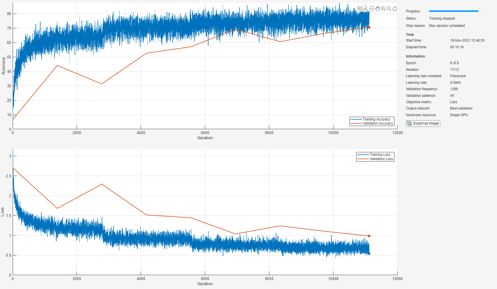
Define trainingOptions (Deep Learning Toolbox) for the CNN. These options are based on [3] and modified through a systematic hyperparameter optimization workflow.

miniBatchSize = 128;
tuneme = 128;
lr = 0.05*miniBatchSize/tuneme;
options = trainingOptions( ...
    "sgdm", ...
    Momentum=0.9, ...
    L2Regularization=0.005, ...
    ...
    MiniBatchSize=miniBatchSize, ...
    MaxEpochs=8, ...
    Shuffle="every-epoch", ...
    ...
    Plots="training-progress", ...
    Verbose=false, ...
    Metrics="accuracy", ...
    ...
    InitialLearnRate=lr, ...
    LearnRateSchedule="piecewise", ...
    LearnRateDropPeriod=2, ...
    LearnRateDropFactor=0.2, ...
    ...
    ValidationData={xTest,yTest}, ...
    ValidationFrequency=floor(size(xTrain,4)/miniBatchSize));

Call trainnet to train the network.

trainedNet = trainnet(xTrain,yTrain,layers,"crossentropy",options);

Evaluate CNN

Call minibatchpredict to predict responses from the trained network using the held-out test set.

cnnResponsesPerSegment = minibatchpredict(trainedNet,xTest);

Average the responses over each 10-second audio clip.

classes = unique(trainLabels);
numFiles = numel(testLabels);

counter = 1;
cnnResponses = zeros(numFiles,numel(classes));
for channel = 1:numFiles
    cnnResponses(channel,:) = sum(cnnResponsesPerSegment(counter:counter+numSegmentsPer10seconds-1,:),1)/numSegmentsPer10seconds;
    counter = counter + numSegmentsPer10seconds;
end

For each 10-second audio clip, choose the maximum of the predictions, then map it to the corresponding predicted location.

[~,classIdx] = max(cnnResponses,[],2);
cnnPredictedLabels = classes(classIdx);

Call confusionchart (Deep Learning Toolbox) to visualize the accuracy on the test set.

figure(Units="normalized",Position=[0.2 0.2 0.5 0.5])
confusionchart(testLabels,cnnPredictedLabels, ...
    title=["Test Accuracy - CNN","Average Accuracy = " + mean(testLabels==cnnPredictedLabels)*100], ...
    ColumnSummary="column-normalized",RowSummary="row-normalized");

Feature Extraction for Ensemble Classifier

Wavelet scattering has been shown in [4] to provide a good representation of acoustic scenes. Define a waveletScattering object. The invariance scale and quality factors were determined through trial and error.

sf = waveletScattering(SignalLength=size(data,1), ...
                       SamplingFrequency=fs, ...
                       InvarianceScale=0.75, ...
                       QualityFactors=[4 1]);

Convert the audio signal to mono, and then call featureMatrix to return the scattering coefficients for the scattering decomposition framework, sf.

dataMono = mean(data,2);
scatteringCoeffients = featureMatrix(sf,dataMono,Transform="log");

Average the scattering coefficients over the 10-second audio clip.

featureVector = mean(scatteringCoeffients,2);
disp("Number of wavelet features per 10-second clip = " + numel(featureVector));

Number of wavelet features per 10-second clip = 286

The helper function HelperWaveletFeatureVector performs the above steps. Use a transform datastore to parallelize the feature extraction. Extract wavelet feature vectors for the train and test sets.

scatteringTrain = transform(adsTrain,@(x)HelperWaveletFeatureVector(x,sf));
xTrain = readall(scatteringTrain,UseParallel=canUseParallelPool);
xTrain = (reshape(xTrain,numel(featureVector),[]))';

scatteringTest = transform(adsTest,@(x)HelperWaveletFeatureVector(x,sf));
xTest = readall(scatteringTest,UseParallel=canUseParallelPool);
xTest = (reshape(xTest,numel(featureVector),[]))';

Define and Train Ensemble Classifier

Use fitcensemble to create a trained classification ensemble model (ClassificationEnsemble).

subspaceDimension = min(150,size(xTrain,2) - 1);
numLearningCycles = 30;
classificationEnsemble = fitcensemble(xTrain,trainLabels, ...
    Method="Subspace", ...
    NumLearningCycles=numLearningCycles, ...
    Learners="discriminant", ...
    NPredToSample=subspaceDimension, ...
    ClassNames=removecats(unique(trainLabels)));

Evaluate Ensemble Classifier

For each 10-second audio clip, call predict to return the labels and the weights, then map it to the corresponding predicted location. Call confusionchart (Deep Learning Toolbox) to visualize the accuracy on the test set.

[waveletPredictedLabels,waveletResponses] = predict(classificationEnsemble,xTest);

figure(Units="normalized",Position=[0.2 0.2 0.5 0.5])
confusionchart(testLabels,waveletPredictedLabels, ...
    title=["Test Accuracy - Wavelet Scattering","Average Accuracy = " + mean(testLabels==waveletPredictedLabels)*100], ...
    ColumnSummary="column-normalized",RowSummary="row-normalized");

fprintf('Average accuracy of classifier = %0.2f\n',mean(testLabels==waveletPredictedLabels)*100)

Average accuracy of classifier = 75.74

Apply Late Fusion

For each 10-second clip, calling predict on the wavelet classifier and the CNN returns a vector indicating the relative confidence in their decision. Multiply the waveletResponses with the cnnResponses to create a late fusion system.

fused = waveletResponses.*cnnResponses;
[~,classIdx] = max(fused,[],2);

predictedLabels = classes(classIdx);

Evaluate Late Fusion

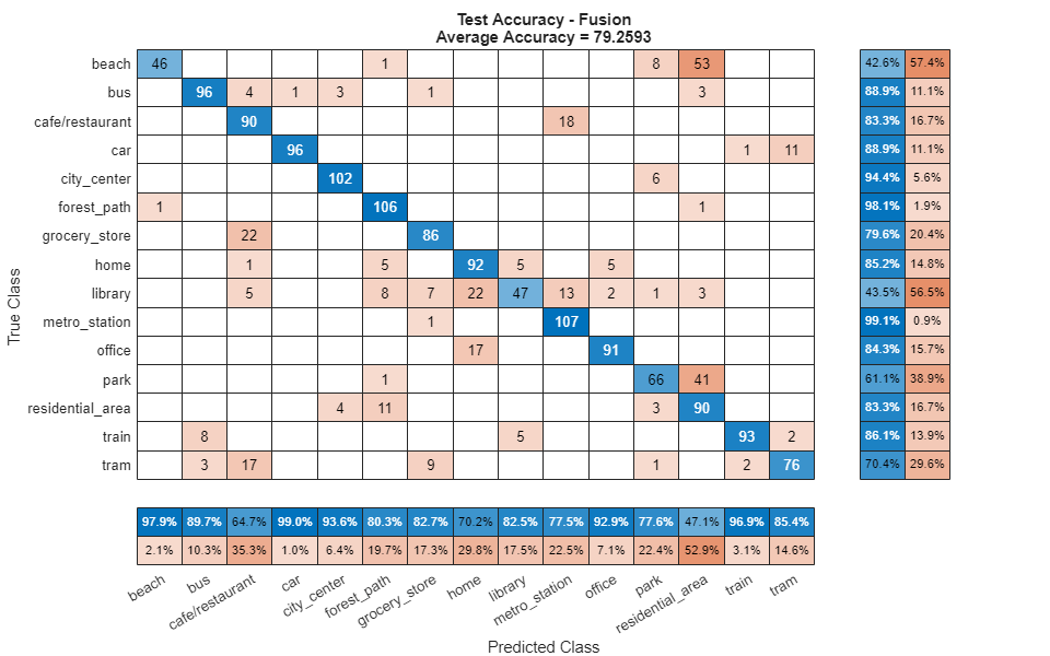
Call confusionchart to visualize the fused classification accuracy.

figure(Units="normalized",Position=[0.2 0.2 0.5 0.5])
confusionchart(testLabels,predictedLabels, ...
    Title=["Test Accuracy - Fusion","Average Accuracy = " + mean(testLabels==predictedLabels)*100], ...
    ColumnSummary="column-normalized",RowSummary="row-normalized");

Supporting Functions

HelperSegmentedMelSpectrograms

function X = HelperSegmentedMelSpectrograms(x,fs,options)
% Copyright 2019-2023 The MathWorks, Inc.

arguments
    x
    fs
    options.WindowLength = 1024
    options.HopLength = 512
    options.NumBands = 128
    options.SegmentLength = 1
    options.SegmentOverlap = 0
    options.FFTLength = 1024
end


x = [sum(x,2),x(:,1)-x(:,2)];
x = x./max(max(x));

[xb_m,~] = buffer(x(:,1),round(options.SegmentLength*fs),round(options.SegmentOverlap*fs),"nodelay");
[xb_s,~] = buffer(x(:,2),round(options.SegmentLength*fs),round(options.SegmentOverlap*fs),"nodelay");
xb = zeros(size(xb_m,1),size(xb_m,2)+size(xb_s,2));
xb(:,1:2:end) = xb_m;
xb(:,2:2:end) = xb_s;

spec = melSpectrogram(xb,fs, ...
    Window=hamming(options.WindowLength,"periodic"), ...
    OverlapLength=options.WindowLength - options.HopLength, ...
    FFTLength=options.FFTLength, ...
    NumBands=options.NumBands, ...
    FrequencyRange=[0,floor(fs/2)], ...
    ApplyLog=true);

X = reshape(spec,size(spec,1),size(spec,2),size(x,2),[]);
end

HelperWaveletFeatureExtractor

function features = HelperWaveletFeatureVector(x,sf)
% Copyright 2019-2023 The MathWorks, Inc.
if canUseGPU
    x = gpuArray(x);
end
x = mean(x,2);
features = featureMatrix(sf,x,Transform="log");
features = gather(mean(features,2));
end

References

[1] A. Mesaros, T. Heittola, and T. Virtanen. Acoustic Scene Classification: an Overview of DCASE 2017 Challenge Entries. In proc. International Workshop on Acoustic Signal Enhancement, 2018.

[2] Huszar, Ferenc. "Mixup: Data-Dependent Data Augmentation." InFERENCe. November 03, 2017. Accessed January 15, 2019. https://www.inference.vc/mixup-data-dependent-data-augmentation/.

[3] Han, Yoonchang, Jeongsoo Park, and Kyogu Lee. "Convolutional neural networks with binaural representations and background subtraction for acoustic scene classification." the Detection and Classification of Acoustic Scenes and Events (DCASE) (2017): 1-5.

[4] Lostanlen, Vincent, and Joakim Anden. Binaural scene classification with wavelet scattering. Technical Report, DCASE2016 Challenge, 2016.

[5] A. J. Eronen, V. T. Peltonen, J. T. Tuomi, A. P. Klapuri, S. Fagerlund, T. Sorsa, G. Lorho, and J. Huopaniemi, "Audio-based context recognition," IEEE Trans. on Audio, Speech, and Language Processing, vol 14, no. 1, pp. 321-329, Jan 2006.

[6] TUT Acoustic scenes 2017, Development dataset

[7] TUT Acoustic scenes 2017, Evaluation dataset