Cardiac Left Ventricle Segmentation from Cine-MRI Images Using U-Net Network
This example shows how to perform semantic segmentation of the left ventricle from 2-D cardiac MRI images using U-Net.
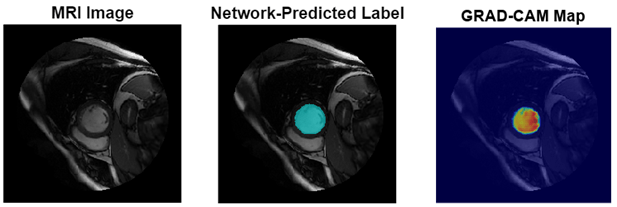
Semantic segmentation associates each pixel in an image with a class label. Segmentation of cardiac MRI images is useful for detecting abnormalities in heart structure and function. A common challenge of medical image segmentation is class imbalance, meaning the region of interest is small relative to the image background. Therefore, the training images contain many more background pixels than labeled pixels, which can limit classification accuracy. In this example, you address class imbalance by using a generalized Dice loss function [1]. You also use the gradient-weighted class activation mapping (Grad-CAM) deep learning explainability technique to determine which regions of an image are important for the pixel classification decision.
This figure shows an example of a cine-MRI image before segmentation, the network-predicted segmentation map, and the corresponding Grad-CAM map.

Load Pretrained Network
Download the pretrained U-Net network by using the downloadTrainedNetwork helper function. The helper function is attached to this example as a supporting file. You can use this pretrained network to run the example without training the network.
exampleDir = fullfile(tempdir,"cardiacMR");
if ~isfolder(exampleDir)
    mkdir(exampleDir);
end

trainedNetworkURL = "https://ssd.mathworks.com/supportfiles" + ...
    "/medical/pretrainedLeftVentricleSegmentationModel_v2.zip";
downloadTrainedNetwork(trainedNetworkURL,exampleDir);
Load the network.
data = load(fullfile(exampleDir,"pretrainedLeftVentricleSegmentationModel_v2.mat"));
trainedNet = data.trainedNet;
Perform Semantic Segmentation
Use the pretrained network to predict the left ventricle segmentation mask for a test image.
Download Data Set
This example uses a subset of the Sunnybrook Cardiac Data data set [2,3]. The subset consists of 45 cine-MRI images and their corresponding ground truth label images. The MRI images were acquired from multiple patients with various cardiac pathologies. The ground truth label images were manually drawn by experts [2]. The MRI images are in the DICOM file format and the label images are in the PNG file format. The total size of the subset of data is ~105 MB.
Download the data set from the MathWorks® website and unzip the downloaded folder.
zipFile = matlab.internal.examples.downloadSupportFile("medical","CardiacMRI.zip");
filepath = fileparts(zipFile);
unzip(zipFile,filepath)
The imageDir folder contains the downloaded and unzipped data set.
imageDir = fullfile(filepath,"Cardiac MRI");Predict Left Ventricle Mask
Read an image from the data set and preprocess the image by using the preprocessImage helper function, which is defined at the end of this example. The helper function resizes MRI images to the input size of the network and converts them from grayscale to three-channel images.
testImg = dicomread(fullfile(imageDir,"images","SC-HF-I-01","SC-HF-I-01_rawdcm_099.dcm"));
trainingSize = [256 256 3];
data = preprocessImage(testImg,trainingSize);
testImg = data{1};
Predict the left ventricle segmentation mask for the test image using the pretrained network by using the semanticseg (Computer Vision Toolbox) function. Specify the classes to predict as "Background" and "LeftVentricle".
classNames = ["Background","LeftVentricle"];
segmentedImg = semanticseg(testImg,trainedNet,Classes=classNames);
Display the test image and an overlay with the predicted mask as a montage.
overlayImg = labeloverlay(mat2gray(testImg),segmentedImg, ...
    Transparency=0.7, ...
    IncludedLabels="LeftVentricle");
imshowpair(mat2gray(testImg),overlayImg,"montage");

Prepare Data for Training
Create an imageDatastore object to read and manage the MRI images.
dataFolder = fullfile(imageDir,"images");
imds = imageDatastore(dataFolder,...
    IncludeSubfolders=true,...
    FileExtensions=".dcm",...
    ReadFcn=@dicomread);
Create a pixelLabelDatastore (Computer Vision Toolbox) object to read and manage the label images. Specify the same classes to predict as defined in the previous section. The pixel label ID 0 maps to the "Background" class name, and the ID 1 maps to the "LeftVentricle" class name.
disp(classNames)
"Background" "LeftVentricle"
pixIDs = [0,1];

labelFolder = fullfile(imageDir,"labels");
pxds = pixelLabelDatastore(labelFolder,classNames,pixIDs,...
    IncludeSubfolders=true,...
    FileExtensions=".png");
Preprocess the data by using the transform function with custom operations specified by the preprocessImage helper function, which is defined at the end of this example. The helper function resizes the MRI images to the input size of the network and converts them from grayscale to three-channel images.
timds = transform(imds,@(img) preprocessImage(img,trainingSize));
Preprocess the label images by using the transform function with custom operations specified by the preprocesslabels helper function, which is defined at the end of this example. The helper function resizes the label images to the input size of the network.
tpxds = transform(pxds,@(img) preprocessLabels(img,trainingSize));
Combine the transformed image and pixel label datastores to create a CombinedDatastore object.
combinedDS = combine(timds,tpxds);
Partition Data for Training, Validation, and Testing
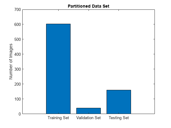
Split the combined datastore into data sets for training, validation, and testing. Allocate 75% of the data for training, 5% for validation, and the remaining 20% for testing.
numImages = numel(imds.Files);
numTrain = round(0.75*numImages);
numVal = round(0.05*numImages);
numTest = round(0.2*numImages);

shuffledIndices = randperm(numImages);
dsTrain = subset(combinedDS,shuffledIndices(1:numTrain));
dsVal = subset(combinedDS,shuffledIndices(numTrain+1:numTrain+numVal));
dsTest = subset(combinedDS,shuffledIndices(numTrain+numVal+1:end));
Visualize the number of images in the training, validation, and testing subsets.
figure
bar([numTrain,numVal,numTest])
title("Partitioned Data Set")
xticklabels({"Training Set","Validation Set","Testing Set"})
ylabel("Number of Images")

Augment Training Data
Augment the training data by using the transform function with custom operations specified by the augmentDataForLVSegmentation helper function, which is defined at the end of this example. The helper function applies random rotations, translations, and reflections to the MRI images and corresponding ground truth labels.
dsTrain = transform(dsTrain,@(data) augmentDataForLVSegmentation(data));
Measure Label Imbalance
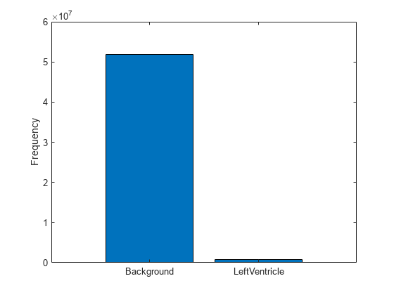
To measure the distribution of class labels in the data set, use the countEachLabel function to count the background pixels and the labeled ventricle pixels.
pixelLabelCount = countEachLabel(pxds)
pixelLabelCount=2×3 table
          Name           PixelCount    ImagePixelCount
    _________________    __________    _______________

    {'Background'   }    5.1901e+07      5.2756e+07
    {'LeftVentricle'}    8.5594e+05      5.2756e+07
Visualize the labels by class. The image contains many more background pixels than labeled ventricle pixels. The label imbalance can bias the training of the network. You address this imbalance when you design the network.
figure
bar(categorical(pixelLabelCount.Name),pixelLabelCount.PixelCount)
ylabel("Frequency")
Define Network Architecture
This example uses a U-Net network for semantic segmentation. Create a U-Net network with an input size of 256-by-256-by-3 that classifies pixels into two categories corresponding to the background and left ventricle.
numClasses = length(classNames);
net = unet(trainingSize,numClasses);
Replace the input network layer with an imageInputLayer object that normalizes image values between 0 and 1000 to the range [0, 1]. Values less than 0 are set to 0 and values greater than 1000 are set to 1000.
inputlayer = imageInputLayer(trainingSize, ...
    Normalization="rescale-zero-one", ...
    Min=0, ...
    Max=1000, ...
    Name="input");
net = replaceLayer(net,net.Layers(1).Name,inputlayer);
Specify Training Options
Specify the training options by using the trainingOptions function. Train the network using the adam optimization solver. Set the learning rate to 0.001 over the span of training. You can experiment with the mini-batch size based on your GPU memory. Batch normalization layers are less effective for smaller values of the mini-batch size. Tune the initial learning rate based on the mini-batch size.
options = trainingOptions("adam", ...
        InitialLearnRate=0.0002,...
        GradientDecayFactor=0.999,...
        L2Regularization=0.0005, ...
        MaxEpochs=100, ...
        MiniBatchSize=32, ...
        Shuffle="every-epoch", ...
        Verbose=false,...
        VerboseFrequency=100,...
        ValidationData=dsVal,...
        Plots="training-progress",...
        ExecutionEnvironment="auto",...
        ResetInputNormalization=false);
Train Network
To train the network, set the doTraining variable to true. Train the network by using the trainnet function. To address the class imbalance between the smaller ventricle regions and larger background, specify a custom loss function, generalizedDiceLoss, which is defined as a helper function at the end of this example.
Train on a GPU if one is available. Using a GPU requires a Parallel Computing Toolbox™ license and a CUDA®-enabled NVIDIA® GPU.
doTraining =false; if doTraining trainedNet = trainnet(dsTrain,net,@generalizedDiceLoss,options); modelDateTime = string(datetime("now",Format="yyyy-MM-dd-HH-mm-ss")); save(fullfile(exampleDir,"trainedLeftVentricleSegmentation-" ... +modelDateTime+".mat"),"trainedNet"); end
Test Network
Segment each image in the test data set by using the trained network. Specify the same classes to predict as used earlier in this example.
resultsDir = fullfile(exampleDir,"Results");

if ~isfolder(resultsDir)
    mkdir(resultsDir)
end

pxdsResults = semanticseg(dsTest,trainedNet,...
    WriteLocation=resultsDir,...
    Verbose=true,...
    MiniBatchSize=1, ...
    Classes=classNames);
Running semantic segmentation network
-------------------------------------
* Processed 161 images.
Evaluate Segmentation Metrics
Evaluate the network by calculating performance metrics using the evaluateSemanticSegmentation (Computer Vision Toolbox) function. The function computes metrics that compare the labels that the network predicts in pxdsResults to the ground truth labels in pxdsTest.
pxdsTest = dsTest.UnderlyingDatastores{2};
metrics = evaluateSemanticSegmentation(pxdsResults,pxdsTest);
Evaluating semantic segmentation results
----------------------------------------
* Selected metrics: global accuracy, class accuracy, IoU, weighted IoU, BF score.
* Processed 161 images.
* Finalizing... Done.
* Data set metrics:
GlobalAccuracy MeanAccuracy MeanIoU WeightedIoU MeanBFScore
______________ ____________ _______ ___________ ___________
0.99832 0.97511 0.94699 0.99674 0.96869
View the metrics by class by querying the ClassMetrics property of metrics.
metrics.ClassMetrics
ans=2×3 table
                     Accuracy      IoU      MeanBFScore
                     ________    _______    ___________

    Background       0.99905      0.9983      0.99497
    LeftVentricle    0.95116     0.89568      0.94241
Evaluate Dice Score
Evaluate the segmentation accuracy by calculating the Dice score between the predicted and ground truth label images. For each test image, calculate the Dice score for the background label and the ventricle label by using the dice (Image Processing Toolbox) function.
reset(pxdsTest);
reset(pxdsResults);

diceScore = zeros(numTest,numClasses);
for idx = 1:numTest

    prediction = read(pxdsResults);
    groundTruth = read(pxdsTest);

    diceScore(idx,1) = dice(prediction{1}==classNames(1),groundTruth{1}==classNames(1));
    diceScore(idx,2) = dice(prediction{1}==classNames(2),groundTruth{1}==classNames(2));
end
Calculate the mean Dice score over all test images and report the mean values in a table.
meanDiceScore = mean(diceScore);
diceTable = array2table(meanDiceScore', ...
    VariableNames="Mean Dice Score", ...
    RowNames=classNames)
diceTable=2×1 table
                     Mean Dice Score
                     _______________

    Background           0.99915
    LeftVentricle        0.92526
Visualize the Dice scores for each class as a box chart. The middle blue line in the plot shows the median Dice score. The upper and lower bounds of the blue box indicate the 25th and 75th percentiles, respectively. Black whiskers extend to the most extreme data points that are not outliers.
figure
boxchart(diceScore)
title("Test Set Dice Accuracy")
xticklabels(classNames)
ylabel("Dice Coefficient")

Explainability
By using explainability methods like Grad-CAM, you can see which areas of an input image the network uses to make its pixel classifications. Use Grad-CAM to show which areas of a test MRI image the network uses to segment the left ventricle.
Load an image from the test data set and preprocess it using the same operations you use to preprocess the training data. The preprocessImage helper function is defined at the end of this example.
testImg = dicomread(fullfile(imageDir,"images","SC-HF-I-01","SC-HF-I-01_rawdcm_099.dcm"));
data = preprocessImage(testImg,trainingSize);
testImg = data{1};
Load the corresponding ground truth label image and preprocess it using the same operations you use to preprocess the training data. The preprocessLabels function is defined at the end of this example.
testGroundTruth = imread(fullfile(imageDir,"labels","SC-HF-I-01","SC-HF-I-01gtmask0099.png"));
data = preprocessLabels({testGroundTruth}, trainingSize);
testGroundTruth = data{1};
Segment the test image using the trained network.
prediction = semanticseg(testImg,trainedNet,Classes=classNames);
To use Grad-CAM, you must select a feature layer from which to extract the feature map and a reduction layer from which to extract the output activations. Use analyzeNetwork to find the layers to use with Grad-CAM. In this example, you use the final ReLU layer as the feature layer and the softmax layer as the reduction layer.
analyzeNetwork(trainedNet)
featureLayer = "Decoder-Stage-4-Conv-2";
reductionLayer = "FinalNetworkSoftmax-Layer";
Compute the Grad-CAM map for the test image by using the gradCAM function. Specify the label index as 2 to create the Grad-CAM map for the ventricle label class.
leftVentricleLabelIdx = 2;
gradCAMMap = gradCAM(trainedNet,testImg,leftVentricleLabelIdx,...
    ReductionLayer=reductionLayer,...
    FeatureLayer=featureLayer);
Visualize the test image, the ground truth labels, the network-predicted labels, and the Grad-CAM map for the ventricle. As expected, the area within the ground truth ventricle mask contributes most strongly to the network prediction of the ventricle label.
figure
tiledlayout(2,2)
nexttile
imshow(mat2gray(testImg))
title("Test Image")

nexttile
imshow(labeloverlay(mat2gray(testImg),testGroundTruth))
title("Ground Truth Label")

nexttile
imshow(labeloverlay(mat2gray(testImg),prediction,IncludedLabels="LeftVentricle"))
title("Network-Predicted Label")

nexttile
imshow(mat2gray(testImg))
hold on
imagesc(gradCAMMap,AlphaData=0.5)
title("GRAD-CAM Map")
colormap jet

Supporting Functions
The preprocessImage helper function preprocesses the MRI images using these steps:
Resize the input image to the target size of the network.
Convert grayscale images to three channel images.
Return the preprocessed image in a cell array.
function out = preprocessImage(img,targetSize)
% Copyright 2023 The MathWorks, Inc.

    targetSize = targetSize(1:2);
    img = imresize(img,targetSize);

    if size(img,3) == 1
        img = repmat(img,[1 1 3]);
    end

    out = {img};

end
The preprocessLabels helper function preprocesses label images using these steps:
Resize the input label image to the target size of the network. The function uses nearest neighbor interpolation so that the output is a binary image without partial decimal values.
Return the preprocessed image in a cell array.
function out = preprocessLabels(labels, targetSize)
% Copyright 2023 The MathWorks, Inc.

    targetSize = targetSize(1:2);
    labels = imresize(labels{1},targetSize,"nearest");

    out = {labels};

end
The augmentDataForLVSegmentation helper function randomly applies these augmentations to each input image and its corresponding label image. The function returns the output data in a cell array.
Random rotation between 0 to 180 degrees.
Random translation along the x- and y-axes of -10 to 10 pixels.
Random reflection to flip the image in the x-axis.
function out = augmentDataForLVSegmentation(data)
% Copyright 2023 The MathWorks, Inc.

    img = data{1};
    labels = data{2};
    inputSize = size(img,[1 2]);

    tform = randomAffine2d(...
        Rotation=[-5 5],...
        XTranslation=[-10 10],...
        YTranslation=[-10 10]);

    sameAsInput = affineOutputView(inputSize,tform,BoundsStyle="sameAsInput");
    img = imwarp(img,tform,"linear",OutputView=sameAsInput);
    labels = imwarp(labels,tform,"nearest",OutputView=sameAsInput);

    out = {img,labels};

end
The generalizedDiceLoss helper function specifies a custom loss function based on the generalized Dice similarity coefficient. The Dice similarity coefficient measures the overlap between two segmented images. The Generalized Dice similarity metric is based on Sørensen-Dice similarity, and controls the contribution that each class makes to the similarity by weighting classes by the inverse size of the expected region. For more details, see generalizedDice (Computer Vision Toolbox).
function loss = generalizedDiceLoss(Y,T)
% Copyright 2024 The MathWorks, Inc.

    % Ignore any NaNs introduced to the training data during augmentation
    T(isnan(T)) = 0;

    z = generalizedDice(Y,T);

    % Compute the mean of the Dice loss across the batch
    loss = 1 - mean(z,"all");

end
References
[1] Milletari, Fausto, Nassir Navab, and Seyed-Ahmad Ahmadi. “V-Net: Fully Convolutional Neural Networks for Volumetric Medical Image Segmentation.” In 2016 Fourth International Conference on 3D Vision (3DV), 565–71. Stanford, CA, USA: IEEE, 2016. https://doi.org/10.1109/3DV.2016.79.
[2] Radau, Perry, Yingli Lu, Kim Connelly, Gideon Paul, Alexander J Dick, and Graham A Wright. “Evaluation Framework for Algorithms Segmenting Short Axis Cardiac MRI.” The MIDAS Journal, July 9, 2009. https://doi.org/10.54294/g80ruo.
[3] “Sunnybrook Cardiac Data – Cardiac Atlas Project.” Accessed January 10, 2023. http://www.cardiacatlas.org/studies/sunnybrook-cardiac-data/.
See Also
imageDatastore | pixelLabelDatastore (Computer Vision Toolbox) | subset | combine | transform | unet (Computer Vision Toolbox) | semanticseg (Computer Vision Toolbox) | evaluateSemanticSegmentation (Computer Vision Toolbox) | gradCAM