使用小波分析和深度学习对时间序列分类
此示例说明如何使用连续小波变换 (CWT) 和深度卷积神经网络 (CNN) 对人体心电图 (ECG) 信号进行分类。
从头开始训练深度 CNN 的计算成本很高,并且需要大量的训练数据。在很多应用中,并没有足够数量的训练数据可用,并且人工新建符合实际情况的训练数据也不可行。在这些情况下,利用已基于大型数据集训练的现有神经网络来完成概念相似的任务是可取的。这种对现有神经网络的利用称为迁移学习。在本示例中,我们采用两个深度 CNN(即 GoogLeNet 和 SqueezeNet,它们针对图像识别进行过预训练)基于时频表示对 ECG 波形进行分类。
GoogLeNet 和 SqueezeNet 是深度 CNN,最初是用于将图像分类至 1000 个类别。我们可重用 CNN 的网络架构,以基于时间序列数据的 CWT 图像对 ECG 信号进行分类。本示例中使用的数据可从 PhysioNet 公开获取。
数据描述
在本示例中,您使用从三组人获得的 ECG 数据:心律失常者 (ARR)、充血性心力衰竭者 (CHF) 和正常窦性心律者 (NSR)。您总共使用来自三个 PhysioNet 数据库的 162 份 ECG 录音:MIT-BIH Arrhythmia 数据库 [3][7]、MIT-BIH Normal Sinus Rhythm 数据库 [3] 和 BIDMC Congestive Heart Failure 数据库 [1][3]。更具体地说,使用了心律失常者的 96 份录音、充血性心力衰竭者的 30 份录音和正常窦性心率者的 36 份录音。目标是训练一个分类器来区分 ARR、CHF 和 NSR。
下载数据
第一步是从 GitHub® 存储库下载数据。要从该网站下载数据,请点击 Code,然后选择 Download ZIP。将文件 physionet_ECG_data-main.zip 保存在您拥有写入权限的文件夹中。此示例的说明假设您已在 MATLAB® 中将文件下载到临时目录 tempdir 中。如果您选择将数据下载到不同于 tempdir 的文件夹中,请修改后续的解压缩和加载数据的说明。
从 GitHub 下载数据后,将文件解压缩到临时目录中。
unzip(fullfile(tempdir,"physionet_ECG_data-main.zip"),tempdir)解压缩会在您的临时目录中创建文件夹 physionet-ECG_data-main。此文件夹包含文本文件 README.md 和 ECGData.zip。ECGData.zip 文件包含
ECGData.matModified_physionet_data.txtLicense.txt
ECGData.mat 保存本示例中使用的数据。文本文件 Modified_physionet_data.txt 是 PhysioNet 的复制政策要求的文件,该文件提供数据的来源说明以及对应用于每份 ECG 录音的预处理步骤的说明。
解压缩 physionet-ECG_data-main 中的 ECGData.zip。将数据文件加载到您的 MATLAB 工作区中。
unzip(fullfile(tempdir,"physionet_ECG_data-main","ECGData.zip"), ...
    fullfile(tempdir,"physionet_ECG_data-main"))
load(fullfile(tempdir,"physionet_ECG_data-main","ECGData.mat"))
ECGData 是包含两个字段的结构体数组:Data 和 Labels。Data 字段是一个 162×65536 矩阵,其中每行均为以 128 赫兹采样的一份 ECG 录音。Labels 是一个 162×1 诊断标签元胞数组,Data 的每行对应一个标签。三个诊断类别是:'ARR'、'CHF' 和 'NSR'。
要存储每个类别的预处理数据,首先在 tempdir 内创建一个 ECG 数据目录 dataDir。然后在 'data' 中创建三个子目录,以每个 ECG 类别命名。辅助函数 helperCreateECGDirectories 可用于完成这一工作。helperCreateECGDirectories 接受 ECGData、ECG 数据目录的名称和父目录的名称作为输入参量。您可以用您具有写入权限的另一个目录替换 tempdir。此示例末尾的支持函数部分提供了该辅助函数的源代码。
parentDir = tempdir;
dataDir = "data";
helperCreateECGDirectories(ECGData,parentDir,dataDir)
绘制每个 ECG 类别的表示图。辅助函数 helperPlotReps 用于实现此目的。helperPlotReps 接受 ECGData 作为输入。此示例末尾的支持函数部分提供了该辅助函数的源代码。
helperPlotReps(ECGData)

创建时频表示
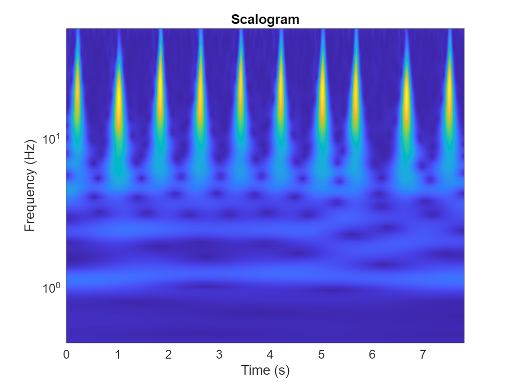
在创建文件夹后,创建 ECG 信号的时频表示。这些表示称为尺度图。尺度图是信号的 CWT 系数的绝对值。
要创建尺度图,请预先计算一个 CWT 滤波器组。当要使用相同的参数获取众多信号的 CWT 时,建议预先计算 CWT 滤波器组。
我们先尝试生成一个尺度图。使用 cwtfilterbank (Wavelet Toolbox) 为具有 1000 个采样的信号创建一个 CWT 滤波器组。使用滤波器组获取信号的前 1000 个采样的 CWT,并基于系数获得尺度图。
Fs = 128;
fb = cwtfilterbank(SignalLength=1000, ...
    SamplingFrequency=Fs, ...
    VoicesPerOctave=12);
sig = ECGData.Data(1,1:1000);
[cfs,frq] = wt(fb,sig);
t = (0:999)/Fs;
figure
pcolor(t,frq,abs(cfs))
set(gca,"yscale","log")
shading interp
axis tight
title("Scalogram")
xlabel("Time (s)")
ylabel("Frequency (Hz)")
使用辅助函数 helperCreateRGBfromTF 将尺度图创建为 RGB 图像,并将其写入 dataDir 中的适当子目录。此辅助函数的源代码在此示例末尾的支持函数部分提供。为了与 GoogLeNet 架构兼容,每个 RGB 图像是大小为 224×224×3 的数组。
helperCreateRGBfromTF(ECGData,parentDir,dataDir)
分为训练数据和验证数据
将尺度图图像加载为图像数据存储。imageDatastore 函数自动根据文件夹名称对图像加标签,并将数据存储为 ImageDatastore 对象。通过图像数据存储可以存储大图像数据,包括无法放入内存的数据,并在 CNN 的训练过程中高效分批读取图像。
allImages = imageDatastore(fullfile(parentDir,dataDir), ...
    "IncludeSubfolders",true, ...
    "LabelSource","foldernames");
将图像随机分成两组,一组用于训练,另一组用于验证。使用 80% 的图像进行训练,其余的用于验证。
[imgsTrain,imgsValidation] = splitEachLabel(allImages,0.8,"randomized");
disp("Number of training images: "+num2str(numel(imgsTrain.Files)))
Number of training images: 130
disp("Number of validation images: "+num2str(numel(imgsValidation.Files)))Number of validation images: 32
GoogLeNet
加载
加载预训练的 GoogLeNet 神经网络。如果未安装 Deep Learning Toolbox™ Model for GoogLeNet Network 支持包,软件将在附加功能资源管理器中提供所需支持包的链接。要安装支持包,请点击链接,然后点击安装。
net = imagePretrainedNetwork("googlenet");从网络中提取并显示层图。
numberOfLayers = numel(net.Layers);
figure("Units","normalized","Position",[0.1 0.1 0.8 0.8])
plot(net)
title("GoogLeNet Layer Graph: "+num2str(numberOfLayers)+" Layers")
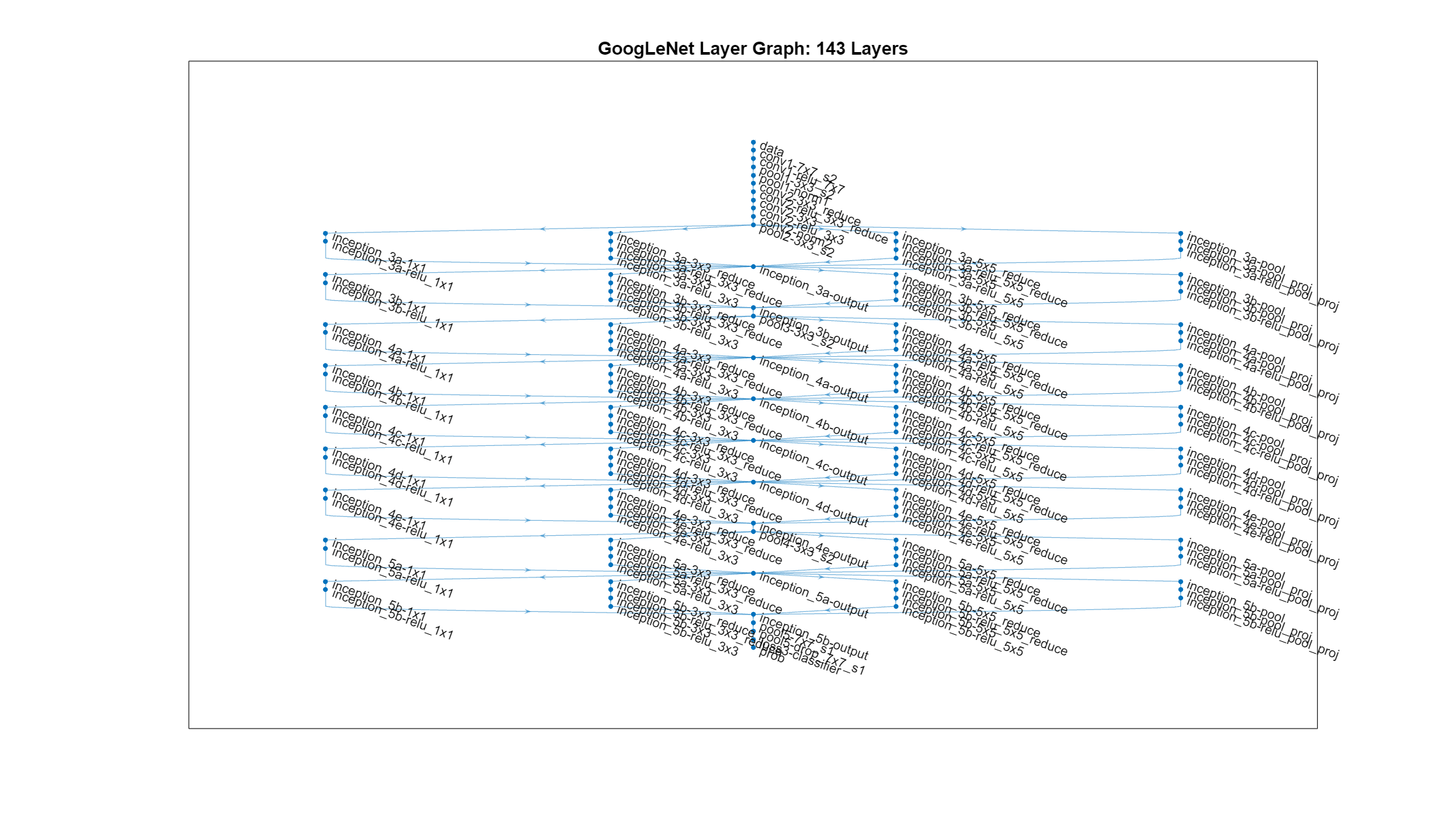
检查网络 Layers 属性的第一个元素。确认 GoogLeNet 需要大小为 224×224×3 的 RGB 图像。
net.Layers(1)
ans =
  ImageInputLayer with properties:

                      Name: 'data'
                 InputSize: [224 224 3]
        SplitComplexInputs: 0

   Hyperparameters
          DataAugmentation: 'none'
             Normalization: 'zerocenter'
    NormalizationDimension: 'auto'
                      Mean: [224×224×3 single]
修改 GoogLeNet 网络参数
网络架构中的每层都可以视为一个滤波器。较浅的层识别图像的更常见特征,如斑点、边缘和颜色。后续层侧重于更具体的特征,以便区分类别。GoogLeNet 经训练可将图像分类至 1000 个目标类别。对于我们的 ECG 分类问题,必须重新训练 GoogLeNet。
检查网络的最后四层。
net.Layers(end-3:end)
ans =
  4×1 Layer array with layers:

     1   'pool5-7x7_s1'        2-D Global Average Pooling   2-D global average pooling
     2   'pool5-drop_7x7_s1'   Dropout                      40% dropout
     3   'loss3-classifier'    Fully Connected              1000 fully connected layer
     4   'prob'                Softmax                      softmax
为防止过拟合,使用了丢弃层。丢弃层以给定的概率将输入元素随机设置为零。有关详细信息,请参阅dropoutLayer。默认概率为 0.5。将网络中的最终丢弃层 pool5-drop_7x7_s1 替换为概率为 0.6 的丢弃层。
newDropoutLayer = dropoutLayer(0.6,"Name","new_Dropout");
net = replaceLayer(net,"pool5-drop_7x7_s1",newDropoutLayer);
网络的卷积层会提取图像特征。然后,GoogLeNet 中的最后一个可学习层 loss3-classifier 包含有关如何将网络提取的特征组合成类概率的信息。要重新训练 GoogLeNet 以对 RGB 图像进行分类,请将其替换为适合数据的新层。
将全连接层 loss3-classifier 替换为新的全连接层,其中滤波器的数量等于类的数量。要使新层中的学习速度快于迁移的层,请增大全连接层的学习率因子。
numClasses = numel(categories(imgsTrain.Labels));
newConnectedLayer = fullyConnectedLayer(numClasses,"Name","new_fc", ...
    "WeightLearnRateFactor",5,"BiasLearnRateFactor",5);
net = replaceLayer(net,"loss3-classifier",newConnectedLayer);
检查最后五层。确认您已替换丢弃层、卷积层和全连接层。
net.Layers(end-3:end)
ans =
  4×1 Layer array with layers:

     1   'pool5-7x7_s1'   2-D Global Average Pooling   2-D global average pooling
     2   'new_Dropout'    Dropout                      60% dropout
     3   'new_fc'         Fully Connected              3 fully connected layer
     4   'prob'           Softmax                      softmax
设置训练选项并训练 GoogLeNet
训练神经网络是一个使损失函数最小的迭代过程。要使损失函数最小,使用梯度下降算法。在每次迭代中,会评估损失函数的梯度并更新下降算法权重。
可以通过设置各种选项来调整训练。InitialLearnRate 指定损失函数负梯度方向的初始步长。MiniBatchSize 指定在每次迭代中使用的训练集子集的大小。一轮指对整个训练集完整运行一遍训练算法。MaxEpochs 指定用于训练的最大轮数。选择正确的轮数至关重要。减少轮数会导致模型欠拟合,而增加轮数会导致过拟合。
使用 trainingOptions 函数指定训练选项。将 MiniBatchSize 设置为 15,MaxEpochs 置为 20,InitialLearnRate 置为 0.0001。通过将 Plots 设置为 training-progress 来可视化训练进度。使用带动量的随机梯度下降优化器。默认情况下,训练在 GPU(如果有)上进行。使用 GPU 需要 Parallel Computing Toolbox™。要查看支持哪些 GPU,请参阅GPU 计算要求 (Parallel Computing Toolbox)。
options = trainingOptions("sgdm", ...
    MiniBatchSize=15, ...
    MaxEpochs=20, ...
    InitialLearnRate=1e-4, ...
    ValidationData=imgsValidation, ...
    ValidationFrequency=10, ...
    Verbose=true, ...
    Plots="training-progress", ...
    Metrics="accuracy");
训练网络。在台式计算机 CPU 上,训练过程通常需要 1-5 分钟。如果您能使用 GPU,运行速度会更快。命令行窗口显示运行期间的训练信息。结果包括验证数据的轮数、迭代序号、历时、小批量准确度、验证准确度和损失函数值。
trainedGN = trainnet(imgsTrain,net,"crossentropy",options); Iteration Epoch TimeElapsed LearnRate TrainingLoss ValidationLoss TrainingAccuracy ValidationAccuracy
_________ _____ ___________ _________ ____________ ______________ ________________ __________________
0 0 00:00:07 0.0001 1.3444 46.875
1 1 00:00:07 0.0001 1.7438 40
10 2 00:00:37 0.0001 1.7555 1.1047 40 62.5
20 3 00:01:03 0.0001 0.75169 0.68252 66.667 68.75
30 4 00:01:27 0.0001 0.74739 0.52126 73.333 78.125
40 5 00:01:50 0.0001 0.49647 0.43025 80 84.375
50 7 00:02:13 0.0001 0.27949 0.36374 93.333 87.5
60 8 00:02:33 0.0001 0.15129 0.36825 93.333 84.375
70 9 00:02:50 0.0001 0.15792 0.29109 100 87.5
80 10 00:03:07 0.0001 0.3697 0.30388 93.333 90.625
90 12 00:03:28 0.0001 0.159 0.25558 100 90.625
100 13 00:03:47 0.0001 0.02107 0.25558 100 90.625
110 14 00:04:06 0.0001 0.17743 0.2531 93.333 90.625
120 15 00:04:27 0.0001 0.086914 0.23932 100 90.625
130 17 00:04:48 0.0001 0.13208 0.24259 93.333 90.625
140 18 00:05:12 0.0001 0.025648 0.20339 100 93.75
150 19 00:05:36 0.0001 0.17878 0.19556 93.333 93.75
160 20 00:06:01 0.0001 0.050998 0.21189 100 93.75
Training stopped: Max epochs completed

评估 GoogLeNet 准确度
使用验证数据评估网络。
classNames = categories(imgsTrain.Labels);
scores = minibatchpredict(trainedGN,imgsValidation);
YPred = scores2label(scores,classNames);
accuracy = mean(YPred==imgsValidation.Labels);
disp("GoogLeNet Accuracy: "+num2str(100*accuracy)+"%")
GoogLeNet Accuracy: 93.75%
精确度与训练可视化图上报告的验证精确度相同。尺度图分成训练集合和验证集合。这两个集合都用于训练 GoogLeNet。评估训练结果的理想方法是让网络对它没有见过的数据进行分类。由于数据量不足,无法分为训练、验证和测试,我们将计算的验证准确度视为网络准确度。
了解 GoogLeNet 激活
CNN 的每层都对输入图像产生响应或激活。然而,一个 CNN 内只有少数几个层适合图像特征提取。检查经过训练的网络的前五层。
trainedGN.Layers(1:5)
ans =
  5×1 Layer array with layers:

     1   'data'             Image Input                   224×224×3 images with 'zerocenter' normalization
     2   'conv1-7x7_s2'     2-D Convolution               64 7×7×3 convolutions with stride [2  2] and padding [3  3  3  3]
     3   'conv1-relu_7x7'   ReLU                          ReLU
     4   'pool1-3x3_s2'     2-D Max Pooling               3×3 max pooling with stride [2  2] and padding [0  1  0  1]
     5   'pool1-norm1'      Cross Channel Normalization   cross channel normalization with 5 channels per element
网络开始的几个层捕获基本的图像特征,如边缘和斑点。要了解这一点,请可视化第一个卷积层的网络滤波器权重。第一个层有 64 组权重。
wghts = trainedGN.Layers(2).Weights;
wghts = rescale(wghts);
wghts = imresize(wghts,8);
figure
I = imtile(wghts,GridSize=[8 8]);
imshow(I)
title("First Convolutional Layer Weights")
通过将激活区域与原始图像进行比较,您可以检查激活区域并发现 GoogLeNet 学习的特征。有关详细信息,请参阅可视化卷积神经网络的激活和可视化卷积神经网络的特征。
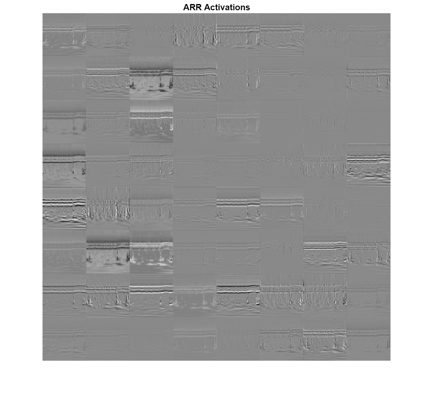
检查卷积层中的哪些区域在来自 ARR 类的图像上激活。与原始图像中的对应区域进行比较。卷积神经网络的每层由许多称为通道的二维数组组成。将网络应用于图像,并检查第一个卷积层 conv1-7x7_s2 的输出激活区域。
convLayer = "conv1-7x7_s2";

imgClass = "ARR";
imgName = "ARR_10.jpg";
imarr = imread(fullfile(parentDir,dataDir,imgClass,imgName));

trainingFeaturesARR = predict(trainedGN,single(imarr),Outputs=convLayer);
sz = size(trainingFeaturesARR);
trainingFeaturesARR = reshape(trainingFeaturesARR,[sz(1) sz(2) 1 sz(3)]);
figure
I = imtile(rescale(trainingFeaturesARR),GridSize=[8 8]);
imshow(I)
title(imgClass+" Activations")
找到此图像的最强通道。将该最强通道与原始图像进行比较。
imgSize = size(imarr);
imgSize = imgSize(1:2);
[~,maxValueIndex] = max(max(max(trainingFeaturesARR)));
arrMax = trainingFeaturesARR(:,:,:,maxValueIndex);
arrMax = rescale(arrMax);
arrMax = imresize(arrMax,imgSize);
figure
I = imtile({imarr,arrMax});
imshow(I)
title("Strongest "+imgClass+" Channel: "+num2str(maxValueIndex))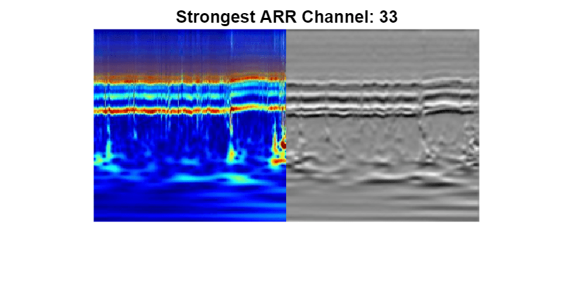
SqueezeNet
SqueezeNet 是一个深度 CNN,其架构支持大小为 227×227×3 的图像。即使 GoogLeNet 的图像大小不同,您也不必以 SqueezeNet 大小生成新 RGB 图像。您可以使用原始的 RGB 图像。
加载
加载预训练的 SqueezeNet 神经网络。
netsqz = imagePretrainedNetwork("squeezenet");从网络中提取层图。确认 SqueezeNet 的层数少于 GoogLeNet。还要确认 SqueezeNet 是针对大小为 227×227×3 的图像配置的。
disp("Number of Layers: "+num2str(numel(netsqz.Layers)))Number of Layers: 68
netsqz.Layers(1)
ans =
  ImageInputLayer with properties:

                      Name: 'data'
                 InputSize: [227 227 3]
        SplitComplexInputs: 0

   Hyperparameters
          DataAugmentation: 'none'
             Normalization: 'zerocenter'
    NormalizationDimension: 'auto'
                      Mean: [1×1×3 single]
修改 SqueezeNet 网络参数
要重新训练 SqueezeNet 对新图像进行分类,请进行与对 GoogLeNet 类似的更改。
检查最后五个网络层。
netsqz.Layers(end-4:end)
ans =
  5×1 Layer array with layers:

     1   'conv10'         2-D Convolution              1000 1×1×512 convolutions with stride [1  1] and padding [0  0  0  0]
     2   'relu_conv10'    ReLU                         ReLU
     3   'pool10'         2-D Global Average Pooling   2-D global average pooling
     4   'prob'           Softmax                      softmax
     5   'prob_flatten'   Flatten                      Flatten
将网络中的最后一个丢弃层替换为概率为 0.6 的丢弃层。
tmpLayer = netsqz.Layers(end-5);
newDropoutLayer = dropoutLayer(0.6,"Name","new_dropout");
netsqz = replaceLayer(netsqz,tmpLayer.Name,newDropoutLayer);
与 GoogLeNet 不同,SqueezeNet 中最后一个可学习层是 1×1 卷积层 conv10,而不是全连接层。将该层替换为新的卷积层,其中滤波器的数量等于类的数量。与对 GoogLeNet 执行的操作一样,增大新层的学习率因子。
numClasses = numel(categories(imgsTrain.Labels));
tmpLayer = netsqz.Layers(end-4);
newLearnableLayer = convolution2dLayer(1,numClasses, ...
        "Name","new_conv", ...
        "WeightLearnRateFactor",10, ...
        "BiasLearnRateFactor",10);
netsqz = replaceLayer(netsqz,tmpLayer.Name,newLearnableLayer);
检查网络的最后五层。确认丢弃层和卷积层已更改。
netsqz.Layers(end-4:end)
ans =
  5×1 Layer array with layers:

     1   'new_conv'       2-D Convolution              3 1×1 convolutions with stride [1  1] and padding [0  0  0  0]
     2   'relu_conv10'    ReLU                         ReLU
     3   'pool10'         2-D Global Average Pooling   2-D global average pooling
     4   'prob'           Softmax                      softmax
     5   'prob_flatten'   Flatten                      Flatten
为 SqueezeNet 准备 RGB 数据
RGB 图像具有适合 GoogLeNet 架构的大小。创建增强的图像数据存储,这些数据存储会自动为 SqueezeNet 架构调整现有 RGB 图像的大小。有关详细信息,请参阅augmentedImageDatastore。
augimgsTrain = augmentedImageDatastore([227 227],imgsTrain);
augimgsValidation = augmentedImageDatastore([227 227],imgsValidation);
设置训练选项并训练 SqueezeNet
创建一组新的用于 SqueezeNet 的训练选项,并训练该网络。
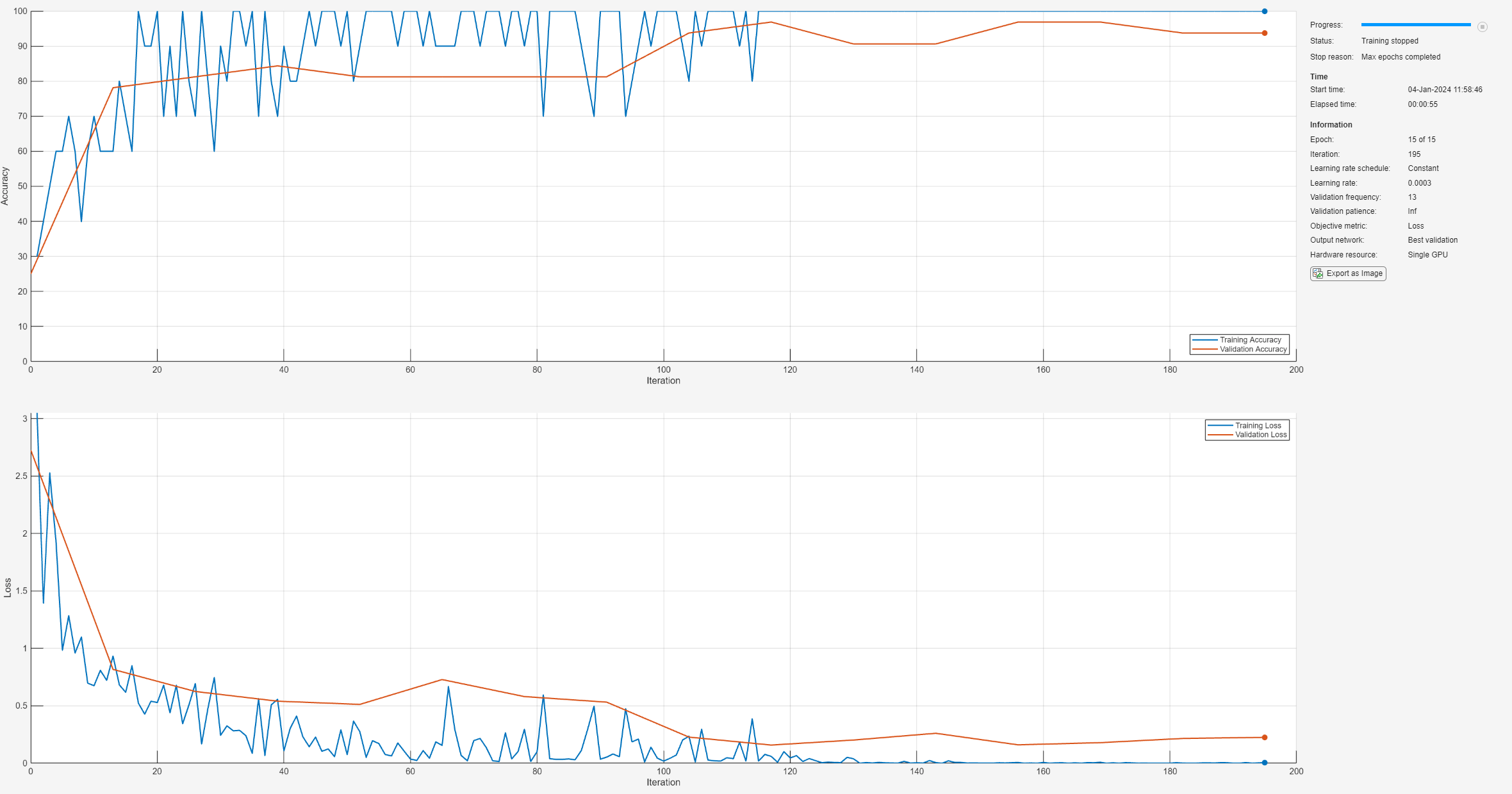
ilr = 3e-4;
miniBatchSize = 10;
maxEpochs = 15;
valFreq = floor(numel(augimgsTrain.Files)/miniBatchSize);
opts = trainingOptions("sgdm", ...
    MiniBatchSize=miniBatchSize, ...
    MaxEpochs=maxEpochs, ...
    InitialLearnRate=ilr, ...
    ValidationData=augimgsValidation, ...
    ValidationFrequency=valFreq, ...
    Verbose=1, ...
    Plots="training-progress", ...
    Metrics="accuracy");

trainedSN = trainnet(augimgsTrain,netsqz,"crossentropy",opts);
    Iteration    Epoch    TimeElapsed    LearnRate    TrainingLoss    ValidationLoss    TrainingAccuracy    ValidationAccuracy
    _________    _____    ___________    _________    ____________    ______________    ________________    __________________
            0        0       00:00:01       0.0003                            2.7267                                        25
            1        1       00:00:01       0.0003          3.0502                                    30
           13        1       00:00:05       0.0003         0.93269           0.81717                  60                78.125
           26        2       00:00:10       0.0003          0.6929           0.62475                  70                 81.25
           39        3       00:00:15       0.0003         0.55664           0.54038                  70                84.375
           50        4       00:00:19       0.0003        0.075004                                   100
           52        4       00:00:20       0.0003         0.27402           0.51236                  90                 81.25
           65        5       00:00:25       0.0003         0.15558           0.72845                  90                 81.25
           78        6       00:00:27       0.0003         0.29531           0.58038                  90                 81.25
           91        7       00:00:30       0.0003        0.053372           0.53191                 100                 81.25
          100        8       00:00:32       0.0003        0.019003                                   100
          104        8       00:00:33       0.0003         0.23475           0.22768                  80                 93.75
          117        9       00:00:37       0.0003        0.059982           0.15849                 100                96.875
          130       10       00:00:43       0.0003        0.038729           0.20219                 100                90.625
          143       11       00:00:46       0.0003       0.0059834           0.26095                 100                90.625
          150       12       00:00:47       0.0003        0.002025                                   100
          156       12       00:00:48       0.0003       0.0067973           0.16036                 100                96.875
          169       13       00:00:50       0.0003       0.0086382           0.17935                 100                96.875
          182       14       00:00:52       0.0003       0.0020118           0.21593                 100                 93.75
          195       15       00:00:54       0.0003       0.0061499           0.22566                 100                 93.75
Training stopped: Max epochs completed
评估 SqueezeNet 准确度
使用验证数据评估网络。
scores = minibatchpredict(trainedSN,augimgsValidation);
YPred = scores2label(scores,classNames);
accuracy = mean(YPred==imgsValidation.Labels);
disp("SqueezeNet Accuracy: "+num2str(100*accuracy)+"%")
SqueezeNet Accuracy: 96.875%
结论
此示例说明如何利用预训练的 CNN(GoogLeNet 和 SqueezeNet)使用迁移学习和连续小波分析对三类 ECG 信号进行分类。ECG 信号的基于小波的时频表示用于创建尺度图。示例生成了尺度图的 RGB 图像。这些图像用于微调这两个深度 CNN。示例还探讨了不同网络层的激活。
利用预训练的 CNN 模型对信号进行分类的方法众多,本示例中介绍的只是其中的一种。也可以使用其他工作流。Deploy Signal Classifier on NVIDIA Jetson Using Wavelet Analysis and Deep Learning (Wavelet Toolbox)和Deploy Signal Classifier Using Wavelets and Deep Learning on Raspberry Pi (Wavelet Toolbox)介绍了如何将代码部署到硬件上进行信号分类。GoogLeNet 和 SqueezeNet 是在 ImageNet 数据库 [10] 子集上预训练的模型,用于 ImageNet Large-Scale Visual Recognition Challenge (ILSVRC) [8] 中。ImageNet 集合包含真实世界物品的图像,例如鱼、鸟、设备和真菌。尺度图不属于现实世界物品的类。为了适应 GoogLeNet 和 SqueezeNet 架构,还对尺度图进行了数据缩减。除了通过微调预训练的 CNN 来对尺度图分类外,也可以选择基于原始尺度图大小从头开始训练 CNN
参考资料
Baim, D. S., W. S. Colucci, E. S. Monrad, H. S. Smith, R. F. Wright, A. Lanoue, D. F. Gauthier, B. J. Ransil, W. Grossman, and E. Braunwald."Survival of patients with severe congestive heart failure treated with oral milrinone."Journal of the American College of Cardiology.Vol. 7, Number 3, 1986, pp. 661–670.
Engin, M."ECG beat classification using neuro-fuzzy network."Pattern Recognition Letters.Vol. 25, Number 15, 2004, pp.1715–1722.
Goldberger A. L., L. A. N. Amaral, L. Glass, J. M. Hausdorff, P. Ch.Ivanov, R. G. Mark, J. E. Mietus, G. B. Moody, C.-K. Peng, and H. E. Stanley."PhysioBank, PhysioToolkit,and PhysioNet:Components of a New Research Resource for Complex Physiologic Signals."Circulation.Vol. 101, Number 23: e215–e220. [Circulation Electronic Pages;
http://circ.ahajournals.org/content/101/23/e215.full]; 2000 (June 13). doi:10.1161/01.CIR.101.23.e215.Leonarduzzi, R. F., G. Schlotthauer, and M. E. Torres."Wavelet leader based multifractal analysis of heart rate variability during myocardial ischaemia."In Engineering in Medicine and Biology Society (EMBC), Annual International Conference of the IEEE, 110–113.Buenos Aires, Argentina:IEEE, 2010.
Li, T., and M. Zhou."ECG classification using wavelet packet entropy and random forests."Entropy.Vol. 18, Number 8, 2016, p.285.
Maharaj, E. A., and A. M. Alonso."Discriminant analysis of multivariate time series:Application to diagnosis based on ECG signals."Computational Statistics and Data Analysis.Vol. 70, 2014, pp. 67–87.
Moody, G. B., and R. G. Mark."The impact of the MIT-BIH Arrhythmia Database."IEEE Engineering in Medicine and Biology Magazine.Vol. 20.Number 3, May-June 2001, pp. 45–50.(PMID: 11446209)
Russakovsky, O., J. Deng, and H. Su et al."ImageNet Large Scale Visual Recognition Challenge."International Journal of Computer Vision.Vol. 115, Number 3, 2015, pp. 211–252.
Zhao, Q., and L. Zhang."ECG feature extraction and classification using wavelet transform and support vector machines."In IEEE International Conference on Neural Networks and Brain, 1089–1092.Beijing, China:IEEE, 2005.
ImageNet.
http://www.image-net.org
支持函数
helperCreateECGDataDirectories 在父目录中创建一个数据目录,然后在该数据目录中创建三个子目录。子目录以 ECGData 中发现的 ECG 信号的每个类命名。
function helperCreateECGDirectories(ECGData,parentFolder,dataFolder)
% This function is only intended to support the ECGAndDeepLearningExample.
% It may change or be removed in a future release.

rootFolder = parentFolder;
localFolder = dataFolder;
mkdir(fullfile(rootFolder,localFolder))

folderLabels = unique(ECGData.Labels);
for i = 1:numel(folderLabels)
    mkdir(fullfile(rootFolder,localFolder,char(folderLabels(i))));
end
end
helperPlotReps 绘制在 ECGData 中发现的 ECG 信号的每个类表示的前一千个采样。
function helperPlotReps(ECGData)
% This function is only intended to support the ECGAndDeepLearningExample.
% It may change or be removed in a future release.

folderLabels = unique(ECGData.Labels);

for k=1:3
    ecgType = folderLabels{k};
    ind = find(ismember(ECGData.Labels,ecgType));
    subplot(3,1,k)
    plot(ECGData.Data(ind(1),1:1000));
    grid on
    title(ecgType)
end
end
helperCreateRGBfromTF 使用 cwtfilterbank (Wavelet Toolbox) 获得 ECG 信号的连续小波变换,并根据小波系数生成尺度图。辅助函数调整尺度图的大小,并将它们作为 jpeg 图像写入磁盘。
function helperCreateRGBfromTF(ECGData,parentFolder,childFolder)
% This function is only intended to support the ECGAndDeepLearningExample.
% It may change or be removed in a future release.

imageRoot = fullfile(parentFolder,childFolder);

data = ECGData.Data;
labels = ECGData.Labels;

[~,signalLength] = size(data);

fb = cwtfilterbank(SignalLength=signalLength,VoicesPerOctave=12);
r = size(data,1);

for ii = 1:r
    cfs = abs(fb.wt(data(ii,:)));
    im = ind2rgb(round(rescale(cfs,0,255)),jet(128));

    imgLoc = fullfile(imageRoot,char(labels(ii)));
    imFileName = char(labels(ii))+"_"+num2str(ii)+".jpg";
    imwrite(imresize(im,[224 224]),fullfile(imgLoc,imFileName));
end
end
另请参阅
cwtfilterbank (Wavelet Toolbox) | imagePretrainedNetwork | trainnet | trainingOptions | dlnetwork | imageDatastore | augmentedImageDatastore