bm
布朗运动 (BM) 模型
说明
创建并显示布朗运动(有时称为算术布朗运动或广义维纳过程)的 bm 对象,该对象来源于 sdeld(以线性形式表示漂移率的 SDE)类。
使用 bm 对象模拟 NVars 个状态变量(由 NBrowns 个风险源驱动)在 NPeriods 个连续观测周期内的样本路径,以便逼近连续时间布朗运动随机过程。这使您能够将 NBrowns 个不相关、零漂移、单方差率布朗分量的向量转换为具有任意漂移、方差率和相关结构的 NVars 个布朗分量的向量。
使用 bm 模拟以下形式的任意向量值布朗运动过程:
其中:
Xt 是过程变量的
NVars×1状态向量。μ 是
NVars×1漂移率向量。V 是
NVars×NBrowns瞬时波动率矩阵。dWt 是(可能)相关的零漂移/单位方差率布朗分量
NBrowns×1向量。
创建对象
描述
BM = bm(___,Name,Value)Name,Value 对组参量指定其他选项来创建一个 bm 对象。
Name 是属性名称,Value 是其对应的值。Name 必须放在单引号 ('') 内。您可以按任意顺序指定多个名称-值对组参量,如 Name1,Value1,…,NameN,ValueN
BM 对象具有以下属性:
StartTime- 初始观测时间StartState-StartTime时的初始状态Correlation-Correlation输入参量的访问函数,可作为时间的函数进行调用Drift- 复合漂移率函数,可作为时间和状态的函数进行调用Diffusion- 复合扩散率函数,可作为时间和状态的函数进行调用Simulation- 模拟函数或方法
输入参量
输出参量
属性
对象函数
interpolate | Brownian interpolation of stochastic differential equations (SDEs) for
SDE, BM, GBM,
CEV, CIR, HWV,
Heston, SDEDDO, SDELD, or
SDEMRD models |
simulate | Simulate multivariate stochastic differential equations (SDEs) for
SDE, BM, GBM,
CEV, CIR, HWV,
Heston, SDEDDO, SDELD,
SDEMRD, Merton, or Bates
models |
simByEuler | Euler simulation of stochastic differential equations (SDEs) for
SDE, BM, GBM,
CEV, CIR, HWV,
Heston, SDEDDO, SDELD, or
SDEMRD models |
simByMilstein | Simulate diagonal diffusion for BM, GBM,
CEV, HWV, SDEDDO,
SDELD, or SDEMRD sample paths by Milstein
approximation |
simByMilstein2 | Simulate BM, GBM, CEV,
HWV, SDEDDO, SDELD,
SDEMRD process sample paths by second order Milstein
approximation |
示例
详细信息
SDE 类之间存在继承关系。
下图是对继承关系的说明。
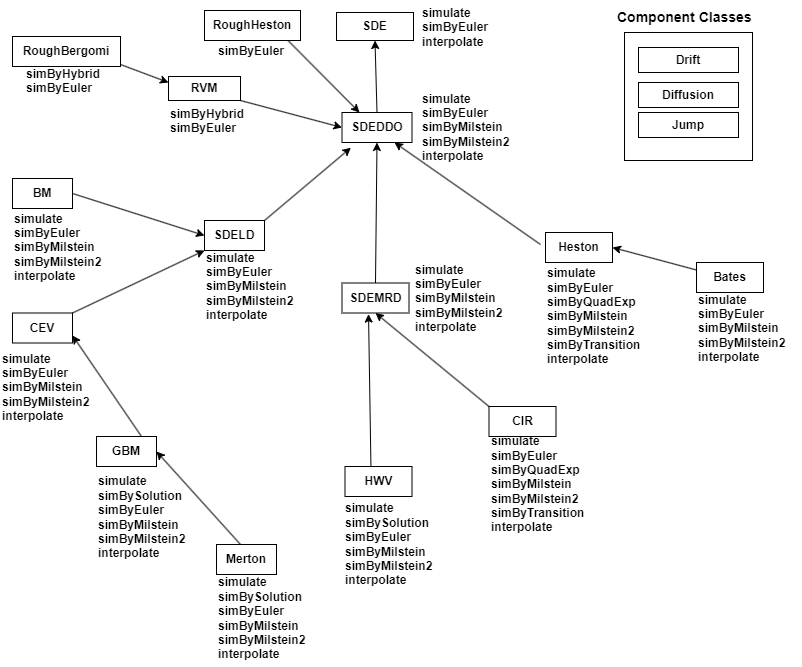
有关详细信息,请参阅 SDE Models、SDE Classes and Associated Simulation Methods 和 SDE 类层次结构。
算法
当您将必需的输入参数指定为数组时,它们将与特定的参数化形式相关联。相比之下,当您将任一必需的输入参数指定为函数时,几乎可以自定义任何设定。
在没有输入的情况下访问输出参数只会返回原始输入设定。因此,当您不带输入调用这些参数时,它们的行为就像简单的属性,您可以测试指定的原始输入的数据类型(是双精度值还是函数,即是静态的还是动态的)。这对于验证和设计方法非常有用。
当您使用输入调用这些参数时,它们的行为类似于函数,给人以动态行为的印象。该参数接受观测时间 t 和状态向量 Xt,并返回适当维度的数组。即使您最初将输入指定为数组,bm 也会将其视为时间和状态的静态函数,这样可以确保所有参数都可由同一接口访问。
参考
[1] Aït-Sahalia, Yacine. “Testing Continuous-Time Models of the Spot Interest Rate.” Review of Financial Studies, vol. 9, no. 2, Apr. 1996, pp. 385–426.
[2] Aït-Sahalia, Yacine. “Transition Densities for Interest Rate and Other Nonlinear Diffusions.” The Journal of Finance, vol. 54, no. 4, Aug. 1999, pp. 1361–95.
[3] Glasserman, Paul. Monte Carlo Methods in Financial Engineering. Springer, 2004.
[4] Hull, John. Options, Futures and Other Derivatives. 7th ed, Prentice Hall, 2009.
[5] Johnson, Norman Lloyd, et al. Continuous Univariate Distributions. 2nd ed, Wiley, 1994.
[6] Shreve, Steven E. Stochastic Calculus for Finance. Springer, 2004.
版本历史记录
在 R2008a 中推出另请参阅
drift | diffusion | sdeld | simulate | interpolate | simByEuler | nearcorr