Price American Basket Options Using Standard Monte Carlo and Quasi-Monte Carlo Simulation

Overview of the Modeling Framework

The ultimate objective of this example is to compare basket option prices derived from different noise processes. The first noise process is a traditional Brownian motion model whose index portfolio price process is driven by correlated Gaussian random draws. As an alternative, the Brownian motion benchmark is compared to noise processes driven by Gaussian and Student's t copulas, referred to collectively as a Brownian copula.

A copula is a multivariate cumulative distribution function (CDF) with uniformly-distributed margins. Although the theoretical foundations were established decades ago, copulas have experienced a tremendous surge in popularity over the last few years, primarily as a technique for modeling non-Gaussian portfolio risks.

Although numerous families exist, all copulas represent a statistical device for modeling the dependence structure between two or more random variables. In addition, important statistics, such as rank correlation and tail dependence are properties of a given copula and are unchanged by monotonic transforms of their margins.

These copula draws produce dependent random variables, which are subsequently transformed to individual variables (margins). This transformation is achieved with a semi-parametric probability distribution with generalized Pareto tails.

The risk-neutral market model to simulate is

where the risk-free rate, r, is assumed constant over the life of the option. Because this is a separable multivariate model, the risk-free return is a diagonal matrix in which the same riskless return is applied to all indices. Dividend yields are ignored to simplify the model and its associated data collection.

In contrast, the specification of the exposure matrix, sigma, depends on how the driving source of uncertainty is modeled. You can model it directly as a Brownian motion (correlated Gaussian random numbers implicitly mapped to Gaussian margins) or model it as a Brownian copula (correlated Gaussian or t random numbers explicitly mapped to semi-parametric margins).

Because the CDF and inverse CDF (quantile function) of univariate distributions are both monotonic transforms, a copula provides a convenient way to simulate dependent random variables whose margins are dissimilar and arbitrarily distributed. Moreover, because a copula defines a given dependence structure regardless of its margins, copula parameter calibration is typically easier than estimation of the joint distribution function.

Once you have simulated sample paths, options are priced by the least squares regression method of Longstaff & Schwartz (see Valuing American Options by Simulation: A Simple Least-Squares Approach, The Review of Financial Studies, Spring 2001). This approach uses least squares to estimate the expected payoff of an option if it is not immediately exercised. It does so by regressing the discounted option cash flows received in the future on the current price of the underlier associated with all in-the-money sample paths. The continuation function is estimated by a simple third-order polynomial, in which all cash flows and prices in the regression are normalized by the option strike price, improving numerical stability.

Import the Supporting Historical Dataset

Load a daily historical dataset of 3-month Euribor, the trading dates spanning the interval 07-Feb-2001 to 24-Apr-2006, and the closing index levels of the following representative large-cap equity indices:

clear
load Data_GlobalIdx2
dates = datetime(dates,'ConvertFrom','datenum');

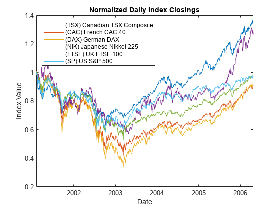
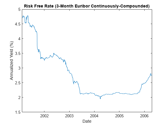
The following plots illustrate this data. Specifically, the plots show the relative price movements of each index and the Euribor risk-free rate proxy. The initial level of each index has been normalized to unity to facilitate the comparison of relative performance over the historical record.

nIndices  = size(Data,2)-1;     % Number of indices

prices = Data(:,1:end-1);

yields = Data(:,end);            % Daily effective yields
yields = 360 * log(1 + yields);  % Continuously-compounded, annualized yield

plot(dates, ret2tick(tick2ret(prices,'Method','continuous'),'Method','continuous'))

xlabel('Date')
ylabel('Index Value')
title ('Normalized Daily Index Closings')
legend(series{1:end-1}, 'Location', 'NorthWest')

plot(dates, 100 * yields)
xlabel('Date')
ylabel('Annualized Yield (%)')
title('Risk Free Rate (3-Month Euribor Continuously-Compounded)')

Extreme Value Theory & Piecewise Probability Distributions

To prepare for copula modeling, characterize individually the distribution of returns of each index. Although the distribution of each return series may be characterized parametrically, it is useful to fit a semi-parametric model using a piecewise distribution with generalized Pareto tails. This uses Extreme Value Theory to better characterize the behavior in each tail.

The Statistics and Machine Learning Toolbox™ software currently supports two univariate probability distributions related to EVT, a statistical tool for modeling the fat-tailed behavior of financial data such as asset returns and insurance losses:

The following analysis highlights the Pareto distribution, which is more widely used in risk management applications.

Suppose we want to create a complete statistical description of the probability distribution of daily asset returns of any one of the equity indices. Assume that this description is provided by a piecewise semi-parametric distribution, where the asymptotic behavior in each tail is characterized by a generalized Pareto distribution.

Ultimately, a copula will be used to generate random numbers to drive the simulations. The CDF and inverse CDF transforms will capture the volatility of simulated returns as part of the diffusion term of the SDE. The mean return of each index is governed by the riskless rate and incorporated in the drift term of the SDE. The following code segment centers the returns (that is, extracts the mean) of each index.

Because the following analysis uses extreme value theory to characterize the distribution of each equity index return series, it is helpful to examine details for a particular country:

returns = tick2ret(prices,'Method','continuous');  % Convert prices to returns
returns = returns - mean(returns);  % Center the returns
index   = 3;                        % Germany stored in column 3

plot(dates(2:end), returns(:,index))
xlabel('Date')
ylabel('Return')
title(['Daily Logarithmic Centered Returns: ' series{index}])

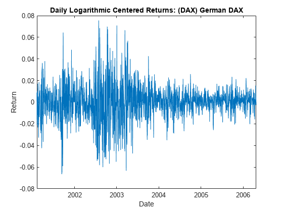
Note that this code segment can be changed to examine details for any country.

Using these centered returns, estimate the empirical, or non-parametric, CDF of each index with a Gaussian kernel. This smoothes the CDF estimates, eliminating the staircase pattern of unsmoothed sample CDFs. Although non-parametric kernel CDF estimates are well-suited for the interior of the distribution, where most of the data is found, they tend to perform poorly when applied to the upper and lower tails. To better estimate the tails of the distribution, apply EVT to the returns that fall in each tail.

Specifically, find the upper and lower thresholds such that 10% of the returns are reserved for each tail. Then fit the amount by which the extreme returns in each tail fall beyond the associated threshold to a Pareto distribution by maximum likelihood.

The following code segment creates one object of type paretotails for each index return series. These Pareto tail objects encapsulate the estimates of the parametric Pareto lower tail, the non-parametric kernel-smoothed interior, and the parametric Pareto upper tail to construct a composite semi-parametric CDF for each index.

tailFraction = 0.1;        % Decimal fraction allocated to each tail
tails = cell(nIndices,1);  % Cell array of Pareto tail objects

for i = 1:nIndices
    tails{i} = paretotails(returns(:,i), tailFraction, 1 - tailFraction, 'kernel');
end

The resulting piecewise distribution object allows interpolation within the interior of the CDF and extrapolation (function evaluation) in each tail. Extrapolation allows estimation of quantiles outside the historical record, which is invaluable for risk management applications.

Pareto tail objects also provide methods to evaluate the CDF and inverse CDF (quantile function), and to query the cumulative probabilities and quantiles of the boundaries between each segment of the piecewise distribution.

Now that three distinct regions of the piecewise distribution have been estimated, graphically concatenate and display the result.

The following code calls the CDF and inverse CDF methods of the Pareto tails object of interest with data other than that upon which the fit is based. The referenced methods have access to the fitted state. They are now invoked to select and analyze specific regions of the probability curve, acting as a powerful data filtering mechanism.

For reference, the plot also includes a zero-mean Gaussian CDF of the same standard deviation. To a degree, the variation in options prices reflect the extent to which the distribution of each asset differs from this normal curve.

minProbability = cdf(tails{index}, (min(returns(:,index))));
maxProbability = cdf(tails{index}, (max(returns(:,index))));

pLowerTail = linspace(minProbability  , tailFraction    , 200); % Lower tail
pUpperTail = linspace(1 - tailFraction, maxProbability  , 200); % Upper tail
pInterior  = linspace(tailFraction    , 1 - tailFraction, 200); % Interior

plot(icdf(tails{index}, pLowerTail), pLowerTail, 'red'  , 'LineWidth', 2)
hold on
grid on
plot(icdf(tails{index}, pInterior) , pInterior , 'black', 'LineWidth', 2)
plot(icdf(tails{index}, pUpperTail), pUpperTail, 'blue' , 'LineWidth', 2)

limits = axis;
x = linspace(limits(1), limits(2));
plot(x, normcdf(x, 0, std(returns(:,index))), 'green', 'LineWidth', 2)

fig = gcf;
fig.Color = [1 1 1];
hold off
xlabel('Centered Return')
ylabel('Probability')
title (['Semi-Parametric/Piecewise CDF: ' series{index}])
legend({'Pareto Lower Tail' 'Kernel Smoothed Interior' ...
        'Pareto Upper Tail' 'Gaussian with Same \sigma'}, 'Location', 'NorthWest')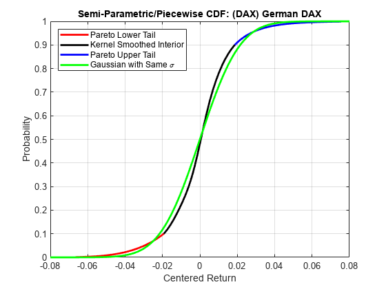

The lower and upper tail regions, displayed in red and blue, respectively, are suitable for extrapolation, while the kernel-smoothed interior, in black, is suitable for interpolation.

Copula Calibration

The Statistics and Machine Learning Toolbox software includes functionality that calibrates and simulates Gaussian and t copulas.

Using the daily index returns, estimate the parameters of the Gaussian and t copulas using the function copulafit. Since a t copula becomes a Gaussian copula as the scalar degrees of freedom parameter (DoF) becomes infinitely large, the two copulas are really of the same family, and therefore share a linear correlation matrix as a fundamental parameter.

Although calibration of the linear correlation matrix of a Gaussian copula is straightforward, the calibration of a t copula is not. For this reason, the Statistics and Machine Learning Toolbox software offers two techniques to calibrate a t copula:

When the uniform variates are transformed by the empirical CDF of each margin, the calibration method is often known as canonical maximum likelihood (CML). The following code segment first transforms the daily centered returns to uniform variates by the piecewise, semi-parametric CDFs derived above. It then fits the Gaussian and t copulas to the transformed data:

U = zeros(size(returns));

for i = 1:nIndices
    U(:,i) = cdf(tails{i}, returns(:,i));    % Transform each margin to uniform
end

options     = statset('Display', 'off', 'TolX', 1e-4);
[rhoT, DoF] = copulafit('t', U, 'Method', 'ApproximateML', 'Options', options);
rhoG        = copulafit('Gaussian', U);

The estimated correlation matrices are quite similar but not identical.

corrcoef(returns)  % Linear correlation matrix of daily returns

ans = 6×6

    1.0000    0.4813    0.5058    0.1854    0.4573    0.6526
    0.4813    1.0000    0.8485    0.2261    0.8575    0.5102
    0.5058    0.8485    1.0000    0.2001    0.7650    0.6136
    0.1854    0.2261    0.2001    1.0000    0.2295    0.1439
    0.4573    0.8575    0.7650    0.2295    1.0000    0.4617
    0.6526    0.5102    0.6136    0.1439    0.4617    1.0000

rhoG               % Linear correlation matrix of the optimized Gaussian copula

rhoG = 6×6

    1.0000    0.4745    0.5018    0.1857    0.4721    0.6622
    0.4745    1.0000    0.8606    0.2393    0.8459    0.4912
    0.5018    0.8606    1.0000    0.2126    0.7608    0.5811
    0.1857    0.2393    0.2126    1.0000    0.2396    0.1494
    0.4721    0.8459    0.7608    0.2396    1.0000    0.4518
    0.6622    0.4912    0.5811    0.1494    0.4518    1.0000

rhoT               % Linear correlation matrix of the optimized t copula

rhoT = 6×6

    1.0000    0.4671    0.4858    0.1907    0.4734    0.6521
    0.4671    1.0000    0.8871    0.2567    0.8500    0.5122
    0.4858    0.8871    1.0000    0.2326    0.7723    0.5877
    0.1907    0.2567    0.2326    1.0000    0.2503    0.1539
    0.4734    0.8500    0.7723    0.2503    1.0000    0.4769
    0.6521    0.5122    0.5877    0.1539    0.4769    1.0000

Note the relatively low degrees of freedom parameter obtained from the t copula calibration, indicating a significant departure from a Gaussian situation.

DoF                % Scalar degrees of freedom parameter of the optimized t copula

DoF = 4.8613

Copula Simulation

Now that the copula parameters have been estimated, simulate jointly-dependent uniform variates using the function copularnd.

Then, by extrapolating the Pareto tails and interpolating the smoothed interior, transform the uniform variates derived from copularnd to daily centered returns via the inverse CDF of each index. These simulated centered returns are consistent with those obtained from the historical dataset. The returns are assumed to be independent in time, but at any point in time possess the dependence and rank correlation induced by the given copula.

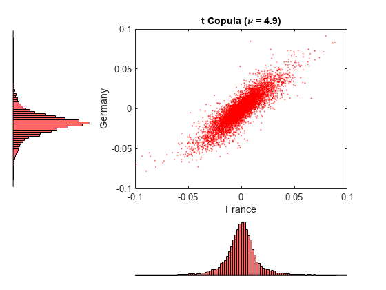
The following code segment illustrates the dependence structure by simulating centered returns using the t copula. It then plots a 2-D scatter plot with marginal histograms for the French CAC 40 and German DAX using the Statistics and Machine Learning Toolbox scatterhist function. The French and German indices were chosen simply because they have the highest correlation of the available data.

nPoints = 10000;                          % Number of simulated observations

s = RandStream.getGlobalStream();
reset(s)

R = zeros(nPoints, nIndices);             % Pre-allocate simulated returns array
U = copularnd('t', rhoT, DoF, nPoints);   % Simulate U(0,1) from t copula

for j = 1:nIndices
    R(:,j) = icdf(tails{j}, U(:,j));
end

h = scatterhist(R(:,2), R(:,3),'Color','r','Marker','.','MarkerSize',1); 
fig = gcf;
fig.Color = [1 1 1];
y1 = ylim(h(1));
y3 = ylim(h(3));
xlim(h(1), [-.1 .1])
ylim(h(1), [-.1 .1])
xlim(h(2), [-.1 .1])
ylim(h(3), [(y3(1) + (-0.1 - y1(1)))  (y3(2) + (0.1 - y1(2)))])
xlabel('France')
ylabel('Germany')
title(['t Copula (\nu = ' num2str(DoF,2) ')'])

Now simulate and plot centered returns using the Gaussian copula.

reset(s)
R = zeros(nPoints, nIndices);             % Pre-allocate simulated returns array
U = copularnd('Gaussian', rhoG, nPoints); % Simulate U(0,1) from Gaussian copula

for j = 1:nIndices
    R(:,j) = icdf(tails{j}, U(:,j));
end

h = scatterhist(R(:,2), R(:,3),'Color','r','Marker','.','MarkerSize',1); 
fig = gcf;
fig.Color = [1 1 1];
y1 = ylim(h(1));
y3 = ylim(h(3));
xlim(h(1), [-.1 .1])
ylim(h(1), [-.1 .1])
xlim(h(2), [-.1 .1])
ylim(h(3), [(y3(1) + (-0.1 - y1(1)))  (y3(2) + (0.1 - y1(2)))])
xlabel('France')
ylabel('Germany')
title('Gaussian Copula')

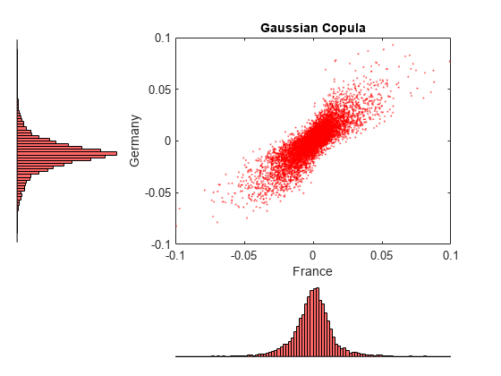
Examine these two figures. There is a strong similarity between the miniature histograms on the corresponding axes of each figure. This similarity is not coincidental.

Both copulas simulate uniform random variables, which are then transformed to daily centered returns by the inverse CDF of the piecewise distribution of each index. Therefore, the simulated returns of any given index are identically distributed regardless of the copula.

However, the scatter graph of each figure indicates the dependence structure associated with the given copula, and in contrast to the univariate margins shown in the histograms, the scatter graphs are distinct.

Once again, the copula defines a dependence structure regardless of its margins, and therefore offers many features not limited to calibration alone.

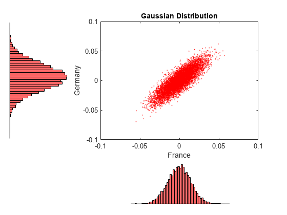
For reference, simulate and plot centered returns using the Gaussian distribution, which underlies the traditional Brownian motion model.

reset(s)
R = mvnrnd(zeros(1,nIndices), cov(returns), nPoints);
h = scatterhist(R(:,2), R(:,3),'Color','r','Marker','.','MarkerSize',1); 
fig = gcf;
fig.Color = [1 1 1];
y1 = ylim(h(1));
y3 = ylim(h(3));
xlim(h(1), [-.1 .1])
ylim(h(1), [-.1 .1])
xlim(h(2), [-.1 .1])
ylim(h(3), [(y3(1) + (-0.1 - y1(1)))  (y3(2) + (0.1 - y1(2)))])
xlabel('France')
ylabel('Germany')
title('Gaussian Distribution')

American Option Pricing Using the Longstaff & Schwartz Approach

Now that the copulas have been calibrated, compare the prices of at-the-money American basket options derived from various approaches. To simply the analysis, assume that:

Now compute the parameters common to all simulation methods:

dt       = 1 / 252;                  % Time increment = 1 day = 1/252 years
yields   = Data(:,end);              % Daily effective yields
yields   = 360 * log(1 + yields);    % Continuously-compounded, annualized yields
r        = mean(yields);             % Historical 3M Euribor average
X        = repmat(100, nIndices, 1); % Initial state vector
strike   = sum(X);                   % Initialize an at-the-money basket

nTrials  = 100;                      % Number of independent trials
nPeriods = 63;  % Number of simulation periods: 63/252 = 0.25 years = 3 months

Now create two separable multi-dimensional market models in which the riskless return and volatility exposure matrices are both diagonal.

While both are diagonal GBM models with identical risk-neutral returns, the first is driven by a correlated Brownian motion and explicitly specifies the sample linear correlation matrix of centered returns. This correlated Brownian motion process is then weighted by a diagonal matrix of annualized index volatilities or standard deviations.

As an alternative, the same model could be driven by an uncorrelated Brownian motion (standard Brownian motion) by specifying correlation as an identity matrix, or by simply accepting the default value. In this case, the exposure matrix sigma is specified as the lower Cholesky factor of the index return covariance matrix. Because the copula-based approaches simulate dependent random numbers, the diagonal exposure form is chosen for consistency. For further details, see Induce Dependence and Correlation Between States.

sigma       = std(returns) * sqrt(252);    % Annualized volatility
correlation = corrcoef(returns);           % Correlated Gaussian disturbances
GBM1        = gbm(diag(r(ones(1,nIndices))), diag(sigma), 'StartState', X, ...
                 'Correlation'             , correlation);

Now create the second model driven by the Brownian copula with an identity matrix sigma.

GBM2 = gbm(diag(r(ones(1,nIndices))), eye(nIndices), 'StartState', X);

The newly created model may seem unusual, but it highlights the flexibility of the SDE architecture.

When working with copulas, it is often convenient to allow the random number generator function Z(t,X) to induce dependence (of which the traditional notion of linear correlation is a special case) with the copula, and to induce magnitude or scale of variation (similar to volatility or standard deviation) with the semi-parametric CDF and inverse CDF transforms. Since the CDF and inverse CDF transforms of each index inherit the characteristics of historical returns, this also explains why the returns are now centered.

In the following sections, statements like:

z = Example_CopulaRNG(returns * sqrt(252), nPeriods, 'Gaussian');

or

z = Example_CopulaRNG(returns * sqrt(252), nPeriods, 't');

fit the Gaussian and t copula dependence structures, respectively, and the semi-parametric margins to the centered returns scaled by the square root of the number of trading days per year (252). This scaling does not annualize the daily centered returns. Instead, it scales them such that the volatility remains consistent with the diagonal annualized exposure matrix sigma of the traditional Brownian motion model (GBM1) created previously.

In this example, you also specify an end-of-period processing function that accepts time followed by state (t,X), and records the sample times and value of the portfolio as the single-unit weighted average of all indices. This function also shares this information with other functions designed to price American options with a constant riskless rate using the least squares regression approach of Longstaff & Schwartz.

f = Example_LongstaffSchwartz(nPeriods, nTrials)

f = struct with fields:
    LongstaffSchwartz: @Example_LongstaffSchwartz/saveBasketPrices
            CallPrice: @Example_LongstaffSchwartz/getCallPrice
             PutPrice: @Example_LongstaffSchwartz/getPutPrice
               Prices: @Example_LongstaffSchwartz/getBasketPrices

Now simulate independent trials of equity index prices over 3 calendar months using the simByEuler method for both a standard Monte Carlo simulation and a Quasi-Monte Carlo simulation. No outputs are requested from the simulation methods; in fact, the simulated prices of the individual indices which comprise the basket are unnecessary. Call option prices are reported for convenience:

reset(s)

simByEuler(GBM1, nPeriods, 'nTrials'  , nTrials, 'DeltaTime', dt, ...
                          'Processes', f.LongstaffSchwartz);

BrownianMotionCallPrice = f.CallPrice(strike, r);
BrownianMotionPutPrice  = f.PutPrice (strike, r);

reset(s)

f = Example_LongstaffSchwartz(nPeriods, nTrials);

simByEuler(GBM1, nPeriods, 'nTrials'  , nTrials, 'DeltaTime', dt, ...
                          'Processes', f.LongstaffSchwartz, ...
                          'MontecarloMethod','quasi');

QuasiMonteCarloCallPrice = f.CallPrice(strike, r);
QuasiMonteCarloPutPrice  = f.PutPrice (strike, r);


reset(s)

z = Example_CopulaRNG(returns * sqrt(252), nPeriods, 'Gaussian');
f = Example_LongstaffSchwartz(nPeriods, nTrials);

simByEuler(GBM2, nPeriods, 'nTrials'  , nTrials, 'DeltaTime', dt, ...
                          'Processes', f.LongstaffSchwartz, 'Z', z);

GaussianCopulaCallPrice = f.CallPrice(strike, r);
GaussianCopulaPutPrice  = f.PutPrice (strike, r);

Now repeat the copula simulation with the t copula dependence structure. You use the same model object for both copulas; only the random number generator and option pricing functions need to be re-initialized.

reset(s)

z = Example_CopulaRNG(returns * sqrt(252), nPeriods, 't');
f = Example_LongstaffSchwartz(nPeriods, nTrials);

simByEuler(GBM2, nPeriods, 'nTrials'  , nTrials, 'DeltaTime', dt, ...
                          'Processes', f.LongstaffSchwartz, 'Z', z);

tCopulaCallPrice = f.CallPrice(strike, r);
tCopulaPutPrice  = f.PutPrice (strike, r);

Finally, compare the American put and call option prices obtained from all models.

disp(' ')

fprintf('                    # of Monte Carlo Trials: %8d\n'    , nTrials)

                    # of Monte Carlo Trials:      100

fprintf('                    # of Time Periods/Trial: %8d\n\n'  , nPeriods)

                    # of Time Periods/Trial:       63

fprintf(' Brownian Motion American Call Basket Price: %8.4f\n'  , BrownianMotionCallPrice)

 Brownian Motion American Call Basket Price:  25.9456

fprintf(' Brownian Motion American Put  Basket Price: %8.4f\n\n', BrownianMotionPutPrice)

 Brownian Motion American Put  Basket Price:  16.4132

fprintf(' Quasi-Monte Carlo American Call Basket Price: %8.4f\n'  , QuasiMonteCarloCallPrice)

 Quasi-Monte Carlo American Call Basket Price:  21.8202

fprintf(' Quasi-Monte Carlo American Put  Basket Price: %8.4f\n\n', QuasiMonteCarloPutPrice)

 Quasi-Monte Carlo American Put  Basket Price:  19.7968

fprintf(' Gaussian Copula American Call Basket Price: %8.4f\n'  , GaussianCopulaCallPrice)

 Gaussian Copula American Call Basket Price:  24.5711

fprintf(' Gaussian Copula American Put  Basket Price: %8.4f\n\n', GaussianCopulaPutPrice)

 Gaussian Copula American Put  Basket Price:  17.4229

fprintf('        t Copula American Call Basket Price: %8.4f\n'  , tCopulaCallPrice)

        t Copula American Call Basket Price:  22.6220

fprintf('        t Copula American Put  Basket Price: %8.4f\n'  , tCopulaPutPrice)

        t Copula American Put  Basket Price:  20.9983

This analysis represents only a small-scale simulation. If the simulation is repeated with 100,000 trials, the following results are obtained:

                  
                   # of Monte Carlo Trials:   100000
                   # of Time Periods/Trial:       63

Brownian Motion American Call Basket Price:  20.0945
Brownian Motion American Put  Basket Price:  16.4808

Quasi-Monte Carlo American Call Basket Price:  20.1935
Quasi-Monte Carlo American Put  Basket Price:  16.4731

Gaussian Copula American Call Basket Price:  20.9183
Gaussian Copula American Put  Basket Price:  16.4416

       t Copula American Call Basket Price:  21.0133
       t Copula American Put  Basket Price:  16.7050

Interestingly, the results agree closely. Put option prices obtained from copulas exceed those of Brownian motion by less than 1%.

A Note on Volatility and Interest Rate Scaling

The same option prices could also be obtained by working with unannualized (in this case, daily) centered returns and riskless rates, where the time increment dt = 1 day rather than 1/252 years. In other words, portfolio prices would still be simulated every trading day; the data is simply scaled differently.

Although not executed, and by first resetting the random stream to its initial internal state, the following code segments work with daily centered returns and riskless rates and produce the same option prices.

Gaussian Distribution/Brownian Motion & Daily Data:

reset(s)

f    = Example_LongstaffSchwartz(nPeriods, nTrials);
GBM1 = gbm(diag(r(ones(1,nIndices))/252), diag(std(returns)), 'StartState', X, ...
          'Correlation', correlation);

simByEuler(GBM1, nPeriods, 'nTrials'  , nTrials, 'DeltaTime', 1, ...
                          'Processes', f.LongstaffSchwartz);

BrownianMotionCallPrice = f.CallPrice(strike, r/252)
BrownianMotionPutPrice  = f.PutPrice (strike, r/252)

reset(s)

f    = Example_LongstaffSchwartz(nPeriods, nTrials);
GBM1 = gbm(diag(r(ones(1,nIndices))/252), diag(std(returns)), 'StartState', X, ...
          'Correlation', correlation);

simByEuler(GBM1, nPeriods, 'nTrials'  , nTrials, 'DeltaTime', dt, ...
                          'Processes', f.LongstaffSchwartz, ...
                          'MontecarloMethod','quasi');

QuasiMonteCarloCallPrice = f.CallPrice(strike, r/252);
QuasiMonteCarloPutPrice  = f.PutPrice (strike, r/252);

Gaussian Copula & Daily Data:

reset(s)

z    = Example_CopulaRNG(returns, nPeriods, 'Gaussian');
f    = Example_LongstaffSchwartz(nPeriods, nTrials);
GBM2 = gbm(diag(r(ones(1,nIndices))/252),   eye(nIndices), 'StartState', X);

simByEuler(GBM2, nPeriods, 'nTrials'  , nTrials, 'DeltaTime',   1, ...
                          'Processes', f.LongstaffSchwartz , 'Z', z);

GaussianCopulaCallPrice = f.CallPrice(strike, r/252)
GaussianCopulaPutPrice  = f.PutPrice (strike, r/252)

t Copula & Daily Data:

reset(s)

z = Example_CopulaRNG(returns, nPeriods, 't');
f = Example_LongstaffSchwartz(nPeriods, nTrials);

simByEuler(GBM2, nPeriods, 'nTrials'  , nTrials, 'DeltaTime',   1, ...
                          'Processes', f.LongstaffSchwartz , 'Z', z);

tCopulaCallPrice = f.CallPrice(strike, r/252)
tCopulaPutPrice  = f.PutPrice (strike, r/252)