roughbergomi

Rough Bergomi model

Since R2024a

Description

Creates and displays a roughbergomi object.

Rough Bergomi models are bivariate composite models, composed of two coupled and dissimilar univariate models, each driven by a single Brownian motion source of risk over NPERIODS consecutive observation periods, approximating continuous-time rough stochastic volatility processes.

The first univariate model is a geometric Brownian motion (GBM) model with a stochastic volatility function, and usually corresponds to a price process whose variance rate is governed by the second univariate model. The second model includes a Volterra process (Riemann-Liouville) which induces the rough behavior of the variance rate (modeling log variance) of the coupled GBM price process.

Creation

Syntax

RoughBergomi = roughbergomi(Return,Alpha,Xi,Eta)

RoughBergomi = roughbergomi(___,Name=Value)

Description

RoughBergomi = roughbergomi(Return,Alpha,Xi,Eta) creates a default RoughBergomi object with Properties for these required arguments.

Specify the required input parameters as one of the following types:

A MATLAB^® array. Specifying an array indicates a static (non-time-varying) parametric specification. This array fully captures all implementation details, which are clearly associated with a parametric form.
A MATLAB function. Specifying a function provides indirect support for virtually any static, dynamic, linear, or nonlinear model. This parameter is supported through an interface because all implementation details are hidden and fully encapsulated by the function.

Note

You can specify combinations of array and function input parameters as needed. Moreover, a parameter is identified as a deterministic function of time if the function accepts a scalar time t as its only input argument. Otherwise, a parameter is assumed to be a function of time t and state X(t) and is invoked with both input arguments.

example

RoughBergomi = roughbergomi(___,Name=Value) creates a RoughBergomi object with additional options specified by one or more name-value arguments to set the properties.

example

Input Arguments

expand all

`Return` — Expected (mean) instantaneous rate of return of GBM price process
scalar numeric | function_handle

Expected (mean) instantaneous rate of return of the GBM price process, specified as an array, a numeric scalar, or a deterministic function of time as a function handle accepting time t or both time t and state X(t).

Data Types: double | function_handle

`Alpha` — Kernel function parameter representing roughness index
scalar numeric

Kernel function parameter representing the roughness index, specified as numeric scalar. The value of Alpha should be in (-0.5, 0.5). The BSS process behaves locally like a fractional Brownian motion (fBm) with the Hurst index H = Alpha + 0.5.

Data Types: double

`Xi` — Forward variance curve
scalar numeric

Forward variance curve specified as an array, a numeric scalar, or a deterministic function of time, Xi must return a scalar when called with a real-valued scalar time t as its only input. Although this function enforces no restrictions, Xi is usually non-negative.

Data Types: double

`Eta` — Volterra `fBm` parameter
scalar numeric > `0`

Volterra fBm parameter, specified as numeric scalar > 0.

Unlike the standard Brownian motion used in traditional models, the fractional Brownian motion (fBm) allows for long memory and roughness in the volatility dynamics. This roughness captures the empirical observation that volatility tends to exhibit slow decay and high-frequency irregularities.

Data Types: double

Name-Value Arguments

Specify optional pairs of arguments as Name1=Value1,...,NameN=ValueN, where Name is the argument name and Value is the corresponding value. Name-value arguments must appear after other arguments, but the order of the pairs does not matter.

Example: RoughBergomi = roughbergomi(Return,Alpha,Xi,Eta,Correlation=0.02)

`StartTime` — Starting time of first observation, applied to all state variables
`0` (default) | scalar

Starting time of the first observation, applied to all state variables, specified as a scalar.

Data Types: double

`StartState` — Initial values of state variables on all trials
`1` (default) | scalar, column vector, or matrix

Initial values of the state variables on all trials, specified as a scalar, column vector, or matrix.

If StartState is a scalar, roughbergomi applies the same initial value to all state variables on all trials.
If StartState is a 2-by-1 column vector, roughbergomi applies a unique initial value to each state variable on all trials.
If StartState is a 2-by-NTRIALS matrix, roughbergomi applies a unique initial value to each state variable on each NTRIALS trials.

Note

Although no restrictions are enforced, for the rough Bergomi model, the StartState of the second variable (variance) is expected to always be 1. The initial forward variance value is specified using Xi.

Data Types: double

`Correlation` — Correlation between Gaussian random variates drawn to generate bivariate Brownian motion vector (Wiener processes)
`2`-by-`2` identity matrix representing independent Gaussian processes (default) | numeric scalar | positive semidefinite matrix | deterministic function

Correlation between Gaussian random variates drawn to generate the bivariate Brownian motion vector (Wiener processes), specified as numeric scalar, a 2-by-2 positive semidefinite matrix, or a deterministic function C(t) that accepts the current time t and returns a 2-by-2 positive semidefinite correlation matrix. If Correlation is not a symmetric positive semidefinite matrix, use nearcorr to create a positive semidefinite matrix for a correlation matrix.

A Correlation matrix represents a static condition.

As a deterministic function of time, Correlation allows you to specify a dynamic correlation structure.

Data Types: double

`Simulation` — User-defined simulation function or SDE simulation method
simulation by Euler approximation (`simByEuler`) (default) | function | SDE simulation method

User-defined simulation function or SDE simulation method, specified as a function or SDE simulation method. The default is simByEuler.

Data Types: function_handle

Properties

expand all

`StartTime` — Starting time of first observation, applied to all state variables
`0` (default) | scalar

Starting time of the first observation, applied to all state variables, returned as a scalar.

Data Types: double

`StartState` — Initial values of state variables
`1` (default) | scalar, column vector, or matrix

Initial values of the state variables, returned as a scalar, column vector, or matrix.

Data Types: double

`Correlation` — Correlation between Gaussian random variates drawn to generate Brownian motion vector (Wiener processes)
`2`-by-`2` identity matrix representing independent Gaussian processes (default) | positive semidefinite matrix

Correlation between Gaussian random variates drawn to generate the Brownian motion vector (Wiener processes), returned as a scalar or positive semidefinite matrix.

Data Types: double

`Return` — Expected (mean) instantaneous rate of return of GBM price process
scalar numeric | function_handle

Expected (mean) instantaneous rate of return of the GBM price process, returned as a numeric scalar or function handle.

Data Types: double | function_handle

`Alpha` — Kernel function parameter representing roughness index
scalar numeric

Kernel function parameter representing roughness index, returned as a numeric scalar.

Data Types: double

`Xi` — Forward variance curve
scalar numeric

Forward variance curve, returned as an array, a numeric scalar, or a deterministic function of time.

Data Types: double

`Eta` — Volterra `fBm` parameter
scalar numeric > `0`

Volterra fBm parameter, specified as numeric scalar > 0.

Data Types: double

Object Functions

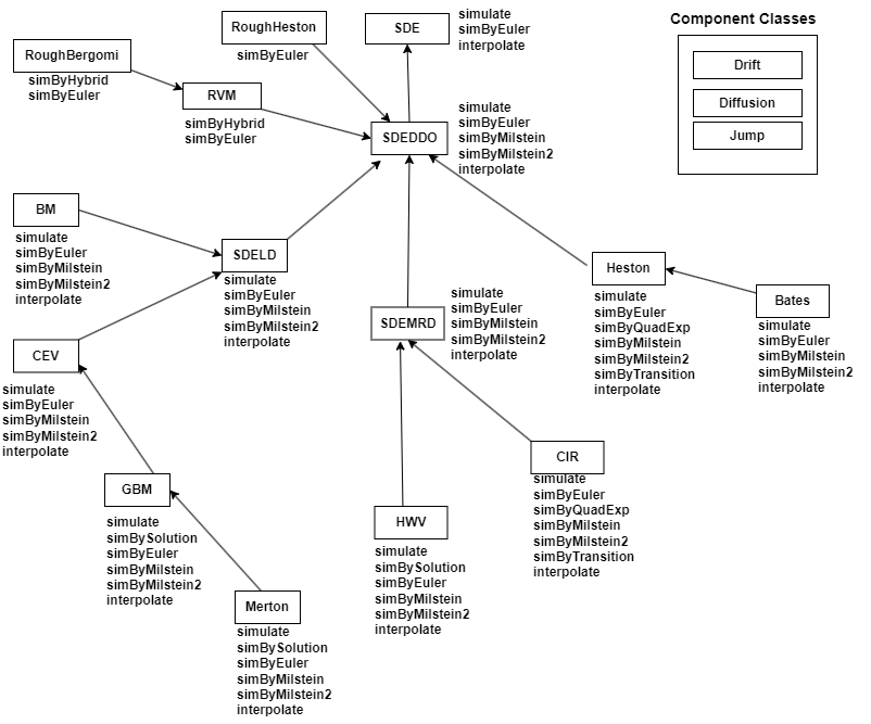
`simByEuler`	Simulate `RVM`, `roughbergomi`, or `roughheston` sample paths by Euler approximation
`simByHybrid`	Simulate `RVM` or `roughbergomi` sample paths by hybrid approximation

Examples

collapse all

Create `roughbergomi` Object

Open Live Script

The roughbergomi object is a bivariate composite model, composed of two coupled and dissimilar univariate models, each driven by a single Brownian motion source of risk over NPERIODS consecutive observation periods, approximating continuous-time rough stochastic volatility processes.

Create a roughbegomi object.

Return = 0.03;
Alpha = -0.03;
Xi = 0.2;
Eta = 0.015;

roughbergomiObj = roughbergomi(Return,Alpha,Xi,Eta)

roughbergomiObj = 
   Class ROUGHBERGOMI: Rough Bergomi
   ----------------------------------------
     Dimensions: State = 2, Brownian = 2
   ----------------------------------------
      StartTime: 0
     StartState: 1 (2x1 double array) 
    Correlation: 2x2 diagonal double array 
         Return: 0.03
          Alpha: -0.03
             Xi: 0.2
            Eta: 0.015

More About

expand all

Instance Hierarchy

There are inheritance relationships among the SDE classes.

The following figure illustrates the inheritance relationships.

For more information, see SDE Models, SDE Classes and Associated Simulation Methods, and SDE Class Hierarchy.

Algorithms

The rough Bergomi model is a type of stochastic volatility model, which means it assumes that the volatility of the underlying asset is not constant but varies over time and is not necessarily correlated with the asset price.

$\begin{array}{l} d X_{1 t} = B (t) X_{1 t} d t + \sqrt{X_{2 t}} X_{1 t} d W_{1 t} \\ X_{2 t} = ξ_{0} (t) e^{η \sqrt{2 a + 1} Y_{t}^{α} - \frac{η^{2}}{2} t^{2 α + 1}} \\ Y_{t} = \int_{0}^{t} {(t - s)}^{α} d W_{s} \end{array}$

The first and second equations represent a geometric Brownian motion (GBM) model with a stochastic volatility function.

The third equation represents the process describing the evolution of the variance rate of the coupled GBM process, where Y_t is a Volterra process. In a Volterra process, the increments are not only dependent on the current state of the process but also on the entire history of the process. This means that the current state of the process is determined by integrating a function over the entire past trajectory of the process, as opposed to just the most recent state.

References

[1] Bayer, C., P. Friz, and J. Gatheral. “Pricing Under Rough Volatility.” Quantitative Finance. Vol. 16, No. 6 , 2016, pp. 887–904.

Version History

Introduced in R2024a

roughbergomi

Description

Creation

Syntax

Description

Input Arguments

`Return` — Expected (mean) instantaneous rate of return of GBM price process
scalar numeric | function_handle

`Alpha` — Kernel function parameter representing roughness index
scalar numeric

`Xi` — Forward variance curve
scalar numeric

`Eta` — Volterra `fBm` parameter
scalar numeric > `0`

`StartTime` — Starting time of first observation, applied to all state variables
`0` (default) | scalar

`StartState` — Initial values of state variables on all trials
`1` (default) | scalar, column vector, or matrix

`Correlation` — Correlation between Gaussian random variates drawn to generate bivariate Brownian motion vector (Wiener processes)
`2`-by-`2` identity matrix representing independent Gaussian processes (default) | numeric scalar | positive semidefinite matrix | deterministic function

`Simulation` — User-defined simulation function or SDE simulation method
simulation by Euler approximation (`simByEuler`) (default) | function | SDE simulation method

Properties

`StartTime` — Starting time of first observation, applied to all state variables
`0` (default) | scalar

`StartState` — Initial values of state variables
`1` (default) | scalar, column vector, or matrix

`Correlation` — Correlation between Gaussian random variates drawn to generate Brownian motion vector (Wiener processes)
`2`-by-`2` identity matrix representing independent Gaussian processes (default) | positive semidefinite matrix

`Return` — Expected (mean) instantaneous rate of return of GBM price process
scalar numeric | function_handle

`Alpha` — Kernel function parameter representing roughness index
scalar numeric

`Xi` — Forward variance curve
scalar numeric

`Eta` — Volterra `fBm` parameter
scalar numeric > `0`

Object Functions

Examples

Create `roughbergomi` Object

More About

Instance Hierarchy

Algorithms

References

Version History

See Also

Topics

roughbergomi

Description

Creation

Syntax

Description

Input Arguments

Return — Expected (mean) instantaneous rate of return of GBM price process scalar numeric | function_handle

Alpha — Kernel function parameter representing roughness index scalar numeric

Xi — Forward variance curve scalar numeric

Eta — Volterra fBm parameter scalar numeric > 0

StartTime — Starting time of first observation, applied to all state variables 0 (default) | scalar

StartState — Initial values of state variables on all trials 1 (default) | scalar, column vector, or matrix

Correlation — Correlation between Gaussian random variates drawn to generate bivariate Brownian motion vector (Wiener processes) 2-by-2 identity matrix representing independent Gaussian processes (default) | numeric scalar | positive semidefinite matrix | deterministic function

Simulation — User-defined simulation function or SDE simulation method simulation by Euler approximation (simByEuler) (default) | function | SDE simulation method

Properties

StartTime — Starting time of first observation, applied to all state variables 0 (default) | scalar

StartState — Initial values of state variables 1 (default) | scalar, column vector, or matrix

Correlation — Correlation between Gaussian random variates drawn to generate Brownian motion vector (Wiener processes) 2-by-2 identity matrix representing independent Gaussian processes (default) | positive semidefinite matrix

Return — Expected (mean) instantaneous rate of return of GBM price process scalar numeric | function_handle

Alpha — Kernel function parameter representing roughness index scalar numeric

Xi — Forward variance curve scalar numeric

Eta — Volterra fBm parameter scalar numeric > 0

Object Functions

Examples

Create roughbergomi Object

More About

Instance Hierarchy

Algorithms

References

Version History

See Also

Topics

`Return` — Expected (mean) instantaneous rate of return of GBM price process
scalar numeric | function_handle

`Alpha` — Kernel function parameter representing roughness index
scalar numeric

`Xi` — Forward variance curve
scalar numeric

`Eta` — Volterra `fBm` parameter
scalar numeric > `0`

`StartTime` — Starting time of first observation, applied to all state variables
`0` (default) | scalar

`StartState` — Initial values of state variables on all trials
`1` (default) | scalar, column vector, or matrix

`Correlation` — Correlation between Gaussian random variates drawn to generate bivariate Brownian motion vector (Wiener processes)
`2`-by-`2` identity matrix representing independent Gaussian processes (default) | numeric scalar | positive semidefinite matrix | deterministic function

`Simulation` — User-defined simulation function or SDE simulation method
simulation by Euler approximation (`simByEuler`) (default) | function | SDE simulation method

`StartTime` — Starting time of first observation, applied to all state variables
`0` (default) | scalar

`StartState` — Initial values of state variables
`1` (default) | scalar, column vector, or matrix

`Correlation` — Correlation between Gaussian random variates drawn to generate Brownian motion vector (Wiener processes)
`2`-by-`2` identity matrix representing independent Gaussian processes (default) | positive semidefinite matrix

`Return` — Expected (mean) instantaneous rate of return of GBM price process
scalar numeric | function_handle

`Alpha` — Kernel function parameter representing roughness index
scalar numeric

`Xi` — Forward variance curve
scalar numeric

`Eta` — Volterra `fBm` parameter
scalar numeric > `0`

Create `roughbergomi` Object