merton
Merton jump diffusion model
Description
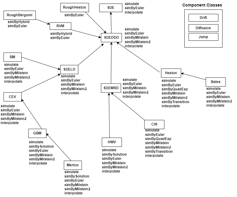
Creates and displays a merton object, which derives from
the gbm object.
The merton model, based on the Merton76 model, allows you to
simulate sample paths of NVars state variables driven by
NBrowns Brownian motion sources of risk and
NJumps compound Poisson processes representing the arrivals of
important events over NPeriods consecutive observation periods. The
simulation approximates continuous-time merton stochastic
processes.
You can simulate any vector-valued merton process of the
form
Here:
Xt is an
NVars-by-1state vector of process variables.B(t,Xt) is an
NVars-by-NVarsmatrix of generalized expected instantaneous rates of return.D(t,Xt)is anNVars-by-NVarsdiagonal matrix in which each element along the main diagonal is the corresponding element of the state vector.V(t,Xt)is anNVars-by-NVarsmatrix of instantaneous volatility rates.dWt is an
NBrowns-by-1Brownian motion vector.Y(t,Xt,Nt)is anNVars-by-NJumpsmatrix-valued jump size function.dNt is an
NJumps-by-1counting process vector.
Creation
Description
Merton = merton(Return,Sigma,JumpFreq,JumpMean,JumpVol)merton object. Specify the required
inputs as one of two types:
MATLAB® array. Specify an array to indicate a static (non-time-varying) parametric specification. This array fully captures all implementation details, which are clearly associated with a parametric form.
MATLAB function. Specify a function to provide indirect support for virtually any static, dynamic, linear, or nonlinear model. This parameter is supported by an interface because all implementation details are hidden and fully encapsulated by the function.
Note
You can specify combinations of array and function input
parameters as needed. Moreover, a parameter is identified as a
deterministic function of time if the function accepts a scalar time
t as its only input argument. Otherwise, a
parameter is assumed to be a function of time t
and state
Xt
and is invoked with both input arguments.
Merton = merton(___,Name,Value)
The merton object has the following Properties:
StartTime— Initial observation timeStartState— Initial state at timeStartTimeCorrelation— Access function for theCorrelationinput argumentDrift— Composite drift-rate functionDiffusion— Composite diffusion-rate functionSimulation— A simulation function or method
Input Arguments
Output Arguments
Properties
Object Functions
simByEuler | Simulate Merton jump diffusion sample paths by Euler
approximation |
simBySolution | Simulate approximate solution of diagonal-drift Merton jump
diffusion process |
simByMilstein | Simulate diagonal diffusion Merton sample paths by Milstein
approximation |
simByMilstein2 | Simulate diagonal diffusion Merton sample paths by second
order Milstein approximation |
simulate | Simulate multivariate stochastic differential equations (SDEs) for
SDE, BM, GBM,
CEV, CIR, HWV,
Heston, SDEDDO, SDELD,
SDEMRD, Merton, or Bates
models |
Examples
More About
Algorithms
The Merton jump diffusion model (Merton 1976) is an extension of the Black-Scholes model, and models sudden asset price movements (both up and down) by adding the jump diffusion parameters with the Poisson process Pt.
Under the risk-neutral measure the model is expressed as follows
Here:
ᵞ is the continuous risk-free rate.
q is the continuous dividend yield.
J is the random percentage jump size conditional on the jump occurring, where
(1+J) has a lognormal distribution:
Here:
μj is the mean of J(μj > -1).
ƛp is the annual frequency (intensity) of the Poisson process Pt (ƛp ≥ 0).
σM is the volatility of the asset price (σM> 0).
Under this formulation, extreme events are explicitly included in the stochastic differential equation as randomly occurring discontinuous jumps in the diffusion trajectory. Therefore, the disparity between observed tail behavior of log returns and that of Brownian motion is mitigated by the inclusion of a jump mechanism.
References
[1] Aït-Sahalia, Yacine. “Testing Continuous-Time Models of the Spot Interest Rate.” Review of Financial Studies 9, no. 2 ( Apr. 1996): 385–426.
[2] Aït-Sahalia, Yacine. “Transition Densities for Interest Rate and Other Nonlinear Diffusions.” The Journal of Finance 54, no. 4 (Aug. 1999): 1361–95.
[3] Glasserman, Paul. Monte Carlo Methods in Financial Engineering. New York: Springer-Verlag, 2004.
[4] Hull, John C. Options, Futures and Other Derivatives. 7th ed, Prentice Hall, 2009.
[5] Johnson, Norman Lloyd, Samuel Kotz, and Narayanaswamy Balakrishnan. Continuous Univariate Distributions. 2nd ed. Wiley Series in Probability and Mathematical Statistics. New York: Wiley, 1995.
[6] Shreve, Steven E. Stochastic Calculus for Finance. New York: Springer-Verlag, 2004.
Version History
Introduced in R2020aSee Also
bates | simByEuler | simBySolution | simulate
Topics
- Simulating Equity Prices
- Simulating Interest Rates
- Stratified Sampling
- Price American Basket Options Using Standard Monte Carlo and Quasi-Monte Carlo Simulation
- Base SDE Models
- Drift and Diffusion Models
- Linear Drift Models
- Parametric Models
- SDEs
- SDE Models
- SDE Class Hierarchy
- Quasi-Monte Carlo Simulation
- Performance Considerations
