Model Progressive Addition Lens Using Presbyopic Eye Model

R2026b

Since R2026b

This example uses:

Optical Design and Simulation Library for Image Processing Toolbox Optical Design and Simulation Library for Image Processing Toolbox

This example shows how to combine a freeform progressive addition lens (PAL) with a presbyopic eye model to analyze retinal image quality across gaze angles. As the eye rotates downward from distance viewing to reading, it looks through progressively stronger zones of the spectacle lens. The progressive surface is a simplified model that illustrates corridor design and spectacle-eye coupling.

Compute Base Radii for Progressive Lens

Optical power varies across the progressive lens surface:

Top, distance zone — Corrects hyperopia. For example, +2 D.
Bottom, near zone — Adds reading power. For example, +2 D of add power over the top zone, for +4 D total.
Corridor — Smoothly transitions between the top and bottom zones.
Sides — unwanted astigmatism from the power gradient.

To model this spectacle lens, define the material and blank parameters. Choose B270 crown glass as the lens material by using the searchGlassLibrary function.

glassTbl = searchGlassLibrary(NameHint="B270",NdRange=[1.52 1.53]);
lensMaterial = glassTbl.Material(1);
nLens = lensMaterial.Nd;
vLens = lensMaterial.Vd;

Define the lens geometry parameters.

lensSD = 25;
lensThickness = 4;

Set the distance prescription for hyperopia and the near addition power in diopters. The add power is the additional power required for near objects in the lower part of the lens.

distancePower = 2.0;
addPower = 2.0;

In a meniscus spectacle lens, both surfaces curve the same way. The front surface power is the base curve, which is 6 D for a mid-range prescription. The back surface power is the base curve minus the distance power, so the net lens power, defined as the front power minus the back power, equals the distance power. To compute the radii from single-surface power, use the formula R = (n – 1)/P from [2].

baseCurve = 6;
backCurve = baseCurve - distancePower;
rFront = (nLens-1)*1000/baseCurve;
rBack = (nLens-1)*1000/backCurve;
disp("Front: " + baseCurve + " D (R = " + rFront + " mm)")

Front: 6 D (R = 87.18 mm)

disp("Back: " + backCurve + " D (R = " + rBack + " mm)")

Back: 4 D (R = 130.77 mm)

disp("Net power: " + baseCurve + " - " + backCurve ...
    + " = +" + distancePower + " D")

Net power: 6 - 4 = +2 D

Model Progressive Freeform Surface

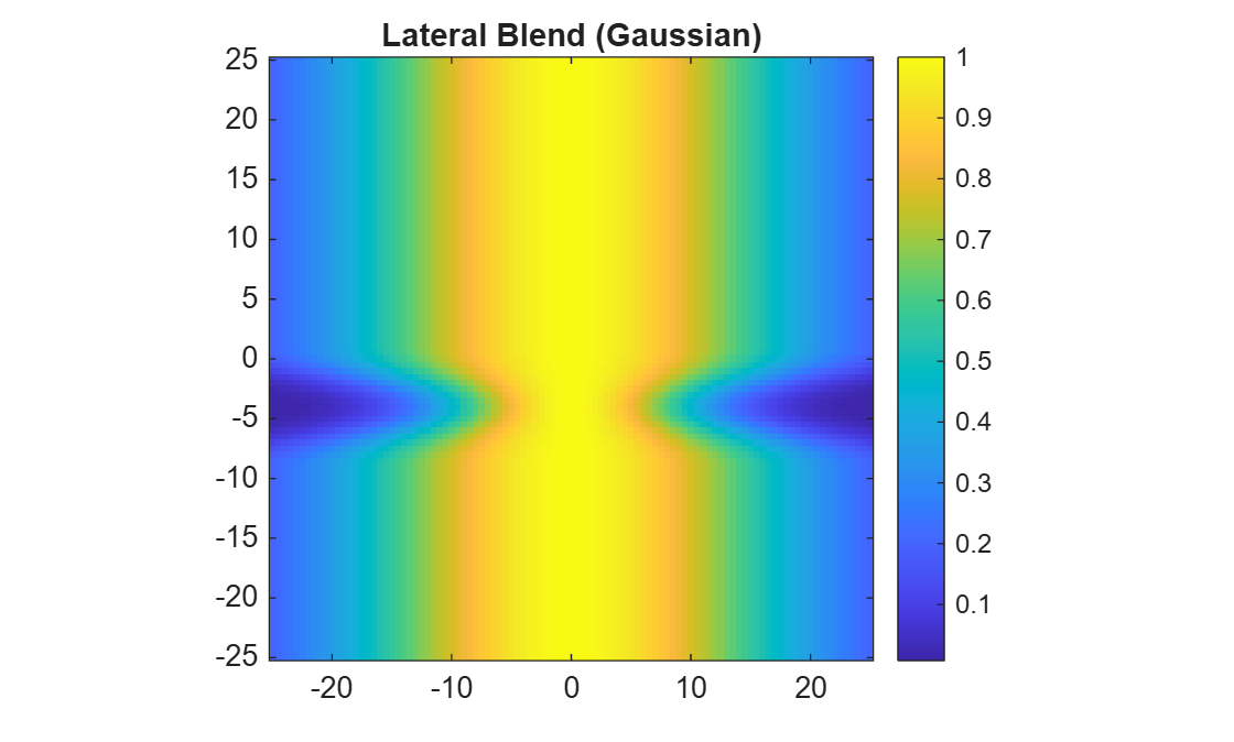
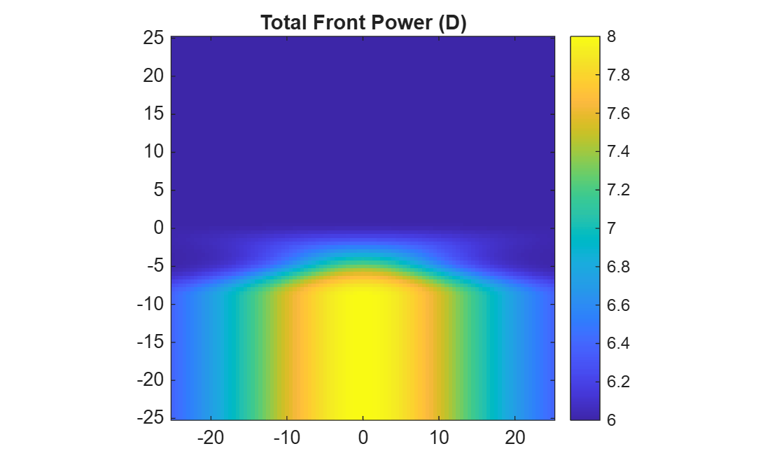
The progressive front surface is freeform, defined by a sag deviation grid rather than a rotationally symmetric shape. The add power smoothly transitions following a raised cosine from zero in the distance zone to the full addition in the near zone along a central corridor. A Gaussian lateral blend confines the add to the corridor center, leaving the periphery at distance curvature with unavoidable astigmatism from the power gradient.

Specify the corridor parameters.

corridorLength = 10;
corridorMidOffset = -4;
yDist = corridorMidOffset + corridorLength/2;
yNear = corridorMidOffset - corridorLength/2;

Compute a raised cosine blend that transitions the add power from zero in the distance zone to full strength in the near zone.

gridSize = 101;
[X,Y] = meshgrid(linspace(-lensSD,lensSD,gridSize));
corridorBlend = max(0,min(1,(yDist-Y)/(yDist-yNear)));
blend = 0.5*(1-cos(pi*corridorBlend));

Visualize the vertical blend to confirm a smooth transition from the distance to the near zone.

imagesc([-lensSD lensSD],[-lensSD lensSD],blend)
axis xy equal tight
colorbar
title("Vertical Blend")

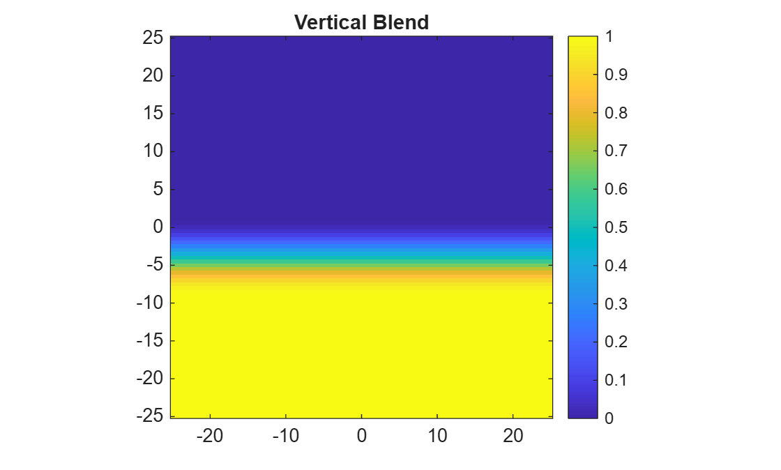
Figure contains an axes object. The axes object with title Vertical Blend contains an object of type image.

Corridor width narrows at mid-corridor where the power gradient is steepest. Compute the Gaussian lateral blend to confine add power to the center.

corridorWidth = 8+6*(1-blend.*(1-blend)*4);
lateralBlend = exp(-0.5*(X./corridorWidth).^2);

Visualize the lateral blend.

imagesc([-lensSD lensSD],[-lensSD lensSD],lateralBlend)
axis xy equal tight
colorbar
title("Lateral Blend (Gaussian)")

Figure contains an axes object. The axes object with title Lateral Blend (Gaussian) contains an object of type image.

Compute the combined add power distribution, and visualize the total front power map.

addLocal = addPower*blend.*lateralBlend;
powerMap = baseCurve + addLocal;
imagesc([-lensSD lensSD],[-lensSD lensSD],powerMap)
axis xy equal tight
colorbar
clim([baseCurve baseCurve+addPower])
title("Total Front Power (D)")

Figure contains an axes object. The axes object with title Total Front Power (D) contains an object of type image.

Compute the sag deviation from the base sphere by using the paraxial approximation.

r2 = X.^2 + Y.^2;
gridDeviation = addLocal.*r2/(2*(nLens-1)*1000);
theta = linspace(0,2*pi,200);
boundX = lensSD*cos(theta);
boundY = lensSD*sin(theta);

Create Spectacle Optical System

Define the position-of-wear parameters that specify how the spectacle frame sits on the face.

vertexDistance = 14;
pantoscopicTilt = 0;
wrapAngle = 0;
age = 55;

Position the spectacle lens so the cornea sits at the coordinate origin. This positioning ensures you measure field point positions relative to the cornea in both the bare eye and the combined system. Create a spectacle optical system using the opticalSystem object, and add the progressive front and back surfaces by using the addRefractiveSurface function.

lensToCornea = lensThickness + vertexDistance;
spec = opticalSystem(Name="Progressive Spectacle");
spec.Position = [0 0 -lensToCornea];
addRefractiveSurface(spec,Radius=rFront,Material=lensMaterial, ...
    SemiDiameter=lensSD,DistanceToNext=lensThickness, ...
    Grid=gridDeviation,GridXLims=[-lensSD lensSD],GridYLims=[-lensSD lensSD], ...
    Name="Progressive Front")
addRefractiveSurface(spec,Radius=rBack,SemiDiameter=lensSD, ...
    DistanceToNext=vertexDistance,Name="Progressive Back")
spec.TiltAngles = [pantoscopicTilt wrapAngle 0];

Model a hyperopic (+2 D) presbyopic eye at age 55 with a maximum accommodation of approximately 2 D. The distance zone corrects hyperopia. The add power offsets near vergence. The eye uses residual accommodation for any remaining demand. Create the eye model and combine it with the spectacle lens.

eye = HybridSchematicEye(Age=age,RefractionDiopters=distancePower, ...
    PupilDiameter=4,Accommodation=0);
combined = opticalSystem(Name="Progressive Lens + Hyperopic Eye");
combined.Wavelengths = 555;
combined.PrimaryWavelengthIndex = 1;
add(combined,spec);
add(combined,eye.OpticalSystem,ReferenceFrame="Global");

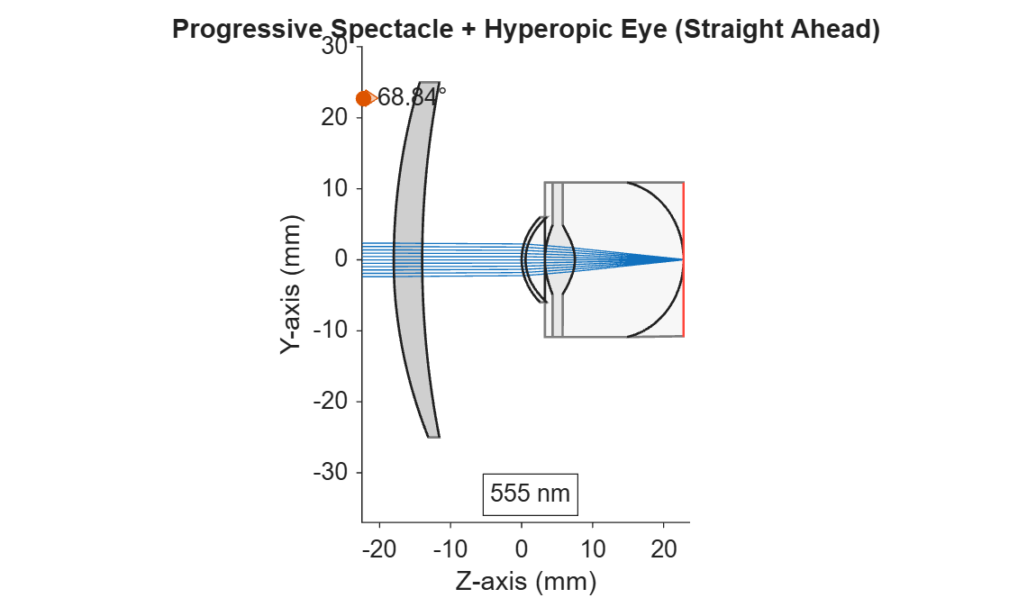
Visualize the combined system by using the view2d function. Trace rays through the system by using the traceRays function, and display them by using the addRays function.

figure
hView = view2d(combined,Title="Progressive Spectacle + Hyperopic Eye (Straight Ahead)")

hView = 
  OpticalSystemViewer2D with properties:

            Title: "Progressive Spectacle + Hyperopic Eye (Straight Ahead)"
    OpticalSystem: [1×1 opticalSystem]
           Labels: "none"
      FieldPoints: "on"
             Rays: [0×0 optics.ui.Rays2D]
           Parent: [1×1 Figure]

  Show all properties

rb = traceRays(combined,Wavelengths=555);
addRays(hView,rb)

Figure contains an object of type optics.ui.opticalsystemviewer2d. The chart of type optics.ui.opticalsystemviewer2d has title Progressive Spectacle + Hyperopic Eye (Straight Ahead).

Compute the on-axis root mean square (RMS) retinal spot size by using the retinalSpot function of the HybridSchematicEye helper object, attached to this example as a supporting file.

rmsOnAxis = HybridSchematicEye.retinalSpot(combined,Wavelengths=555);
disp("On-axis RMS: " + rmsOnAxis*1000 + " um")

On-axis RMS: 23.3214 um

Evaluate Intermediate Gaze

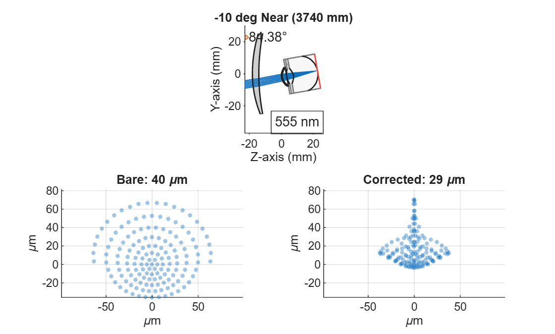
At an intermediate gaze angle, the eye looks through the corridor of the progressive lens. Compare spot size for the bare, uncorrected eye versus the corrected system.

Set the gaze angle to –10 degrees, which means the eye looks downward when facing the negative z-direction.

intermAngle = -10;
readingDist = 3740;
gazeY = readingDist*sind(intermAngle);
gazeZ = -readingDist*cosd(intermAngle);
eyeBare = HybridSchematicEye(Age=age,RefractionDiopters=distancePower, ...
    PupilDiameter=4,GazePoint=[0 gazeY gazeZ]);

To find where the gaze intercepts the progressive front surface, trace the chief ray by using the traceChiefRay function. Define the gaze direction by using the fieldPoint function. Because you do not know the lens accommodation at this point, use zero accommodation.

eyeCorrected = HybridSchematicEye(Age=age,RefractionDiopters=distancePower, ...
    PupilDiameter=4,Accommodation=0,GazePoint=[0 gazeY gazeZ]);
spectacledEye = opticalSystem(Name="Progressive Lens + Eye");
spectacledEye.Wavelengths = 555;
add(spectacledEye,spec);
add(spectacledEye,eyeCorrected.OpticalSystem,ReferenceFrame="Global");
spectacledEye.FieldPoints = fieldPoint(Position=[0 gazeY gazeZ]);

Sample the add power grid at the gaze intercept point, and compute the required additional accommodation. The eye caps this value to the maximum for its age.

chiefRay = traceChiefRay(spectacledEye,Wavelengths=555)

chiefRay = 
  RayBundle with properties:

    FieldPoint: [1×1 optics.fieldpoint.FieldPosition]
    Wavelength: 555
      Sampling: [1×1 struct]
       RayData: [1×1 struct]

yOnLens = chiefRay.RayData.LocalHitPoints(1,1,2);
lensAddAtGaze = interp2(X,Y,addLocal,0,yOnLens);
eyeCorrected.Accommodation = max(0,1000/readingDist-lensAddAtGaze);

Recreate the system with the correctly accommodated eye for this gaze angle and distance.

spectacledEye = opticalSystem(Name="Progressive Lens + Eye");
spectacledEye.Wavelengths = 555;
spectacledEye.PrimaryWavelengthIndex = 1;
add(spectacledEye,spec);
add(spectacledEye,eyeCorrected.OpticalSystem,ReferenceFrame="Global");
spectacledEye.FieldPoints = fieldPoint(Position=[0 gazeY gazeZ]);

Visualize the system, and compare the bare and corrected retinal spots.

tiledlayout(2,2,TileSpacing="compact",Padding="compact");
nexttile([1 2]);
hView = view2d(spectacledEye)

hView = 
  OpticalSystemViewer2D with properties:

            Title: ""
    OpticalSystem: [1×1 opticalSystem]
           Labels: "none"
      FieldPoints: "on"
             Rays: [0×0 optics.ui.Rays2D]
           Parent: [1×1 TiledChartLayout]

  Show all properties

rb = traceRays(spectacledEye,Wavelengths=555);
addRays(hView,rb)
title(intermAngle + " deg Near (" + readingDist + " mm)")
axBare = nexttile;
[rmsBare,spotsBare] = HybridSchematicEye.retinalSpot(eyeBare.OpticalSystem,Wavelengths=555);
scatter(spotsBare(:,1)*1000,spotsBare(:,2)*1000,10,"filled",MarkerFaceAlpha=0.4)
axis equal
grid on
xlabel("\mum")
ylabel("\mum")
title("Bare: " + round(rmsBare*1000) + " \mum")

axCorr = nexttile;
[rmsCorr,spotsCorr] = HybridSchematicEye.retinalSpot(spectacledEye,Wavelengths=555);
scatter(spotsCorr(:,1)*1000,spotsCorr(:,2)*1000,10,"filled",MarkerFaceAlpha=0.4)
axis equal
grid on
xlabel("\mum")
ylabel("\mum")
title("Corrected: " + round(rmsCorr*1000) + " \mum")
linkaxes([axBare,axCorr],"xy")

$Figure contains 2 axes objects and another object of type optics.ui.opticalsystemviewer2d. Axes object 1 with title Bare: 40 mu m, xlabel \mum, ylabel \mum contains an object of type scatter. Axes object 2 with title Corrected: 29 mu m, xlabel \mum, ylabel \mum contains an object of type scatter. The chart of type optics.ui.opticalsystemviewer2d has title -10 deg Near (3740 mm).$

Visualize Intermediate Gaze Position

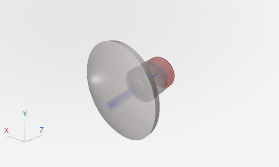
Visualize the system in 3-D by using the view3d function. Trace rays through the system by using the traceRays function, and specify a hexapolar sampling grid by using the samplingGrid function.

hv3d = view3d(spectacledEye,Title="Intermediate Position (-10 deg, 3740 mm)");
rb = traceRays(spectacledEye,SamplingGrid=samplingGrid("Hexapolar",4));
addRays(hv3d,rb)

Figure Progressive Lens + Eye contains an object of type optics.ui.opticalsystemviewer3d.

Explore Gaze Directions

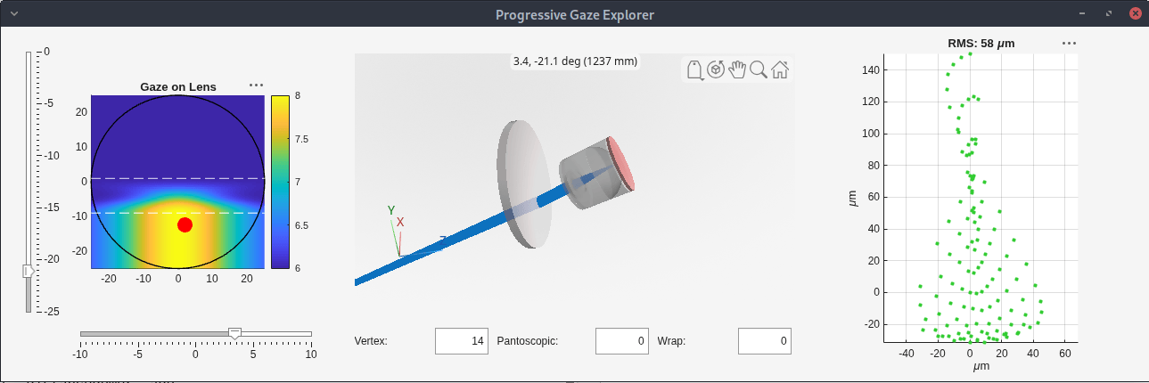
To explore how image quality changes as the eye rotates from distance to near viewing through the progressive zones, you can create a UI by using the gazeExplorer helper function.

gazeExplorer(spec,powerMap,addLocal,X,Y,boundX,boundY, ...
    yDist,yNear,baseCurve,lensThickness,distancePower,age, ...
    vertexDistance,pantoscopicTilt,wrapAngle)

The left pane of the UI shows the gaze point on the lens, indicating the effective power region for that gaze angle. The center pane shows a 3-D visualization of the eye with the spectacle lens and tunable position-of-wear parameters. The right pane shows the spot on the retinal surface. The simplified power blend produces noticeable peripheral astigmatism in the retinal spot.

Gaze explorer UI showing lens power map, 3-D eye model with spectacle lens, and retinal spot diagram for a selected gaze direction.

References

[1] Meister, Darryl J., and Scott W. Fisher. "Progress in the Spectacle Correction of Presbyopia. Part 1: Design and Development of Progressive Lenses." Clinical and Experimental Optometry 91, no. 3 (2008): 240–250. https://doi.org/10.1111/j.1444-0938.2007.00245.x.

[2] Hecht, Eugene. Optics. 5th ed. Pearson, 2017. Chapter 5.

Helper Functions

`gazeExplorer`

Open an interactive UI for exploring how image quality changes across gaze angles through the progressive lens.

function gazeExplorer(spec,powerMap,addLocal,X,Y,boundX,boundY, ...
        yDist,yNear,baseCurve,lensThickness,distancePower,age, ...
        vertexDistance,pantoscopicTilt,wrapAngle)
    fig = uifigure(Name="Progressive Gaze Explorer");
    fig.Position(3:4) = [1400 600];
    gl = uigridlayout(fig,[1 3],ColumnWidth={"1x","1.5x","1x"});
    glGaze = uigridlayout(gl,[2 2], ...
        RowHeight={"1x",40},ColumnWidth={50,"1x"});
    glGaze.Layout.Row = 1;
    glGaze.Layout.Column = 1;
    sldY = uislider(glGaze,Orientation="vertical", ...
        Limits=[-25 0],Value=0);
    sldY.Layout.Row = 1;
    sldY.Layout.Column = 1;
    sldY.MajorTicks = -25:5:0;
    sldX = uislider(glGaze,Limits=[-10 10],Value=0);
    sldX.Layout.Row = 2;
    sldX.Layout.Column = 2;
    sldX.MajorTicks = -15:5:15;
    glMid = uigridlayout(gl,[2 1],RowHeight={"1x",50});
    glMid.Layout.Row = 1;
    glMid.Layout.Column = 2;
    gl3D = uigridlayout(glMid,[1 1]);
    gl3D.Layout.Row = 1;
    glPOW = uigridlayout(glMid,[1 6], ...
        ColumnWidth={80 60 100 60 80 60});
    glPOW.Layout.Row = 2;
    uilabel(glPOW,Text="Vertex:")
    efVertex = uieditfield(glPOW,"numeric",Value=vertexDistance)
    uilabel(glPOW,Text="Pantoscopic:")
    efPanto = uieditfield(glPOW,"numeric",Value=pantoscopicTilt)
    uilabel(glPOW,Text="Wrap:")
    efWrap = uieditfield(glPOW,"numeric",Value=wrapAngle)
    lensToCornea = lensThickness + vertexDistance;
    axSpot = uiaxes(gl);
    axSpot.Layout.Row = 1;
    axSpot.Layout.Column = 3;
    eyeCorrected = HybridSchematicEye(Age=age,RefractionDiopters=distancePower, ...
        PupilDiameter=4,Accommodation=0);
    spectacledEye = opticalSystem(Name="Progressive Lens + Eye");
    spectacledEye.Wavelengths = 555;
    spectacledEye.PrimaryWavelengthIndex = 1;
    add(spectacledEye,spec);
    add(spectacledEye,eyeCorrected.OpticalSystem,ReferenceFrame="Global");
    spectacledEye.FieldPoints = fieldPoint(Angle=[0 0]);
    ax1 = uiaxes(glGaze);
    ax1.Layout.Row = 1;
    ax1.Layout.Column = 2;
    surf(ax1,X,Y,powerMap,EdgeColor="none");
    hold(ax1,"on");
    plot3(ax1,boundX,boundY,max(powerMap(:))*ones(size(boundX)),"k-",LineWidth=1);
    hGazeDot = plot3(ax1,0,0,max(powerMap(:)), ...
        "ro",MarkerSize=12,MarkerFaceColor="r");
    yline(ax1,yDist,"w--",LineWidth=1);
    yline(ax1,yNear,"w--",LineWidth=1);
    hold(ax1,"off");
    view(ax1,0,90)
    axis(ax1,"equal","tight")
    clim(ax1,[baseCurve baseCurve+max(addLocal(:))])
    colorbar(ax1)
    title(ax1,"Gaze on Lens")
    hv3d = view3d(spectacledEye,Parent=gl3D);
    hv3d.Title = "0, 0 deg (6000 mm)";
    [rmsInit,spotsInit] = HybridSchematicEye.retinalSpot(spectacledEye,Wavelengths=555);
    hScatCorr = scatter(axSpot,spotsInit(:,1)*1000,spotsInit(:,2)*1000, ...
        10,[0.2 0.8 0.2],"filled")
    axis(axSpot,"equal")
    grid(axSpot,"on")
    xlabel(axSpot,"\mum")
    ylabel(axSpot,"\mum")
    title(axSpot,"RMS: " + round(rmsInit*1000) + " \mum")
    sldY.ValueChangedFcn = @(~,~) updateGaze();
    sldX.ValueChangedFcn = @(~,~) updateGaze();
    efVertex.ValueChangedFcn = @(~,~) updateGaze();
    efPanto.ValueChangedFcn = @(~,~) updateGaze();
    efWrap.ValueChangedFcn = @(~,~) updateGaze();

    function updateGaze()
        gazeAngleY = sldY.Value;
        gazeAngleX = sldX.Value;
        lensToCornea = lensThickness + efVertex.Value;
        spec.Position = [0 0 -lensToCornea];
        spec.TiltAngles = [efPanto.Value efWrap.Value 0];
        gazeDist = interp1([0 -25],[6000 350],gazeAngleY);
        gazeX = gazeDist*sind(gazeAngleX);
        gazeY = gazeDist*sind(gazeAngleY);
        gazeZ = -gazeDist*cosd(gazeAngleY)*cosd(gazeAngleX);
        eyeCorrected.GazePoint = [gazeX gazeY gazeZ];
        eyeCorrected.Accommodation = 0;
        sysNew = opticalSystem(Name="Progressive Lens + Eye");
        sysNew.Wavelengths = 555;
        sysNew.PrimaryWavelengthIndex = 1;
        add(sysNew,spec)
        add(sysNew,eyeCorrected.OpticalSystem,ReferenceFrame="Global")
        sysNew.FieldPoints = fieldPoint(Position=[gazeX gazeY gazeZ]);
        chiefRay = traceChiefRay(sysNew,Wavelengths=555);
        xOnLens = chiefRay.RayData.LocalHitPoints(1,1,1);
        yOnLens = chiefRay.RayData.LocalHitPoints(1,1,2);
        lensAddAtGaze = interp2(X,Y,addLocal,xOnLens,yOnLens);
        objectVergence = 1000/gazeDist;
        eyeCorrected.Accommodation = max(0,objectVergence-lensAddAtGaze);
        sysNew = opticalSystem(Name="Progressive Lens + Eye");
        sysNew.Wavelengths = 555;
        sysNew.PrimaryWavelengthIndex = 1;
        add(sysNew,spec)
        add(sysNew,eyeCorrected.OpticalSystem,ReferenceFrame="Global")
        sysNew.FieldPoints = fieldPoint(Position=[gazeX gazeY gazeZ]);
        hGazeDot.XData = xOnLens;
        hGazeDot.YData = yOnLens;
        hv3d.OpticalSystem = sysNew;
        hv3d.Title = round(gazeAngleX,1) + ", " + round(gazeAngleY,1) ...
            + " deg (" + round(gazeDist) + " mm)";
        addRays(hv3d,traceRays(sysNew,SamplingGrid=samplingGrid("Hexapolar")))
        [rmsNew,spotsNew] = HybridSchematicEye.retinalSpot(sysNew,Wavelengths=555);
        hScatCorr.XData = spotsNew(:,1)*1000;
        hScatCorr.YData = spotsNew(:,2)*1000;
        axis(axSpot,"equal")
        title(axSpot,"RMS: " + round(rmsNew*1000) + " \mum")
    end
end