Medical Image-Based Finite Element Analysis of Spine

Download Data

This example uses a CT scan saved as a directory of DICOM files. The scan is part of a data set that contains three CT volumes. Run this code to download the data set from the MathWorks website as a zip file and unzip the file. The total size of the data set is approximately 81 MB.

zipFile = matlab.internal.examples.downloadSupportFile("medical","MedicalVolumeDICOMData.zip");
filepath = fileparts(zipFile);
unzip(zipFile,filepath)

After you download and unzip the data set, the scan used in this example is available in the dataFolder directory.

dataFolder = fullfile(filepath,"MedicalVolumeDICOMData","LungCT01");

Segment Vertebra from CT Scan

This example uses a binary segmentation mask of one vertebra in the spine. The mask was created by segmenting the spine from a chest CT scan using the Medical Image Labeler app. For an example of how to segment medical image volumes in the app, see Label 3-D Medical Image Using Medical Image Labeler.

The segmentation mask is attached to this example as a supporting file. Load the mask as a medicalVolume object.

labelVol = medicalVolume("LungCT01.nii.gz");

The VolumeGeometry property of a medical volume object contains a medicalref3d object that defines the patient coordinate system for the scan. Extract the medicalref3d object for the mask into a new variable, R.

R = labelVol.VolumeGeometry;

Extract Vertebra Geometry and Generate FE Mesh

Extract Isosurface of Vertebra Mask

Calculate the isosurface faces and vertices for the vertebra mask by using the extractIsosurface function. The vertices coordinates are in the intrinsic coordinate system defined by rows, columns, and slices.

isovalue = 1;
[faces,vertices] = extractIsosurface(labelVol.Voxels,isovalue);

Transform vertices to the patient coordinate system defined by R by using the intrinsicToWorld object function. The X, Y, and Z outputs define the xyz-coordinates of the surface points, in millimeters.

I = vertices(:,1);
J = vertices(:,2);
K = vertices(:,3);

[X,Y,Z] = intrinsicToWorld(R,I,J,K);
verticesPatient = [X Y Z];

Convert the vertex coordinates to meters.

verticesPatientMeters = verticesPatient.*10^-3;

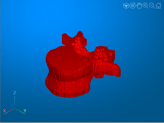
Display the vertebral isosurface as a triangulated Surface object.

triangul = triangulation(double(faces),double(verticesPatientMeters));
viewer = viewer3d;
surface = images.ui.graphics.Surface(viewer,data=triangul,Color=[1 0 0],Alpha=1);

Create PDE Model Geometry

Create a general PDEModel model container for a system of three equations. A general model allows you to assign spatially varying material properties based on bone density.

model = createpde(3);

Specify the geometry for the model by using the geometryFromMesh (Partial Differential Equation Toolbox) object function, with the isosurface in patient coordinates as input.

geometryFromMesh(model,verticesPatientMeters',faces');
pdegplot(model,FaceLabels="on")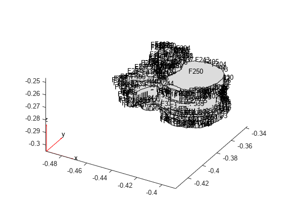

Generate Mesh from Model Geometry

Specify the maximum edge length for the FE mesh elements. This example uses a max edge length of 1.6 mm, which was determined using a mesh convergence analysis.

hMax = 0.0016;

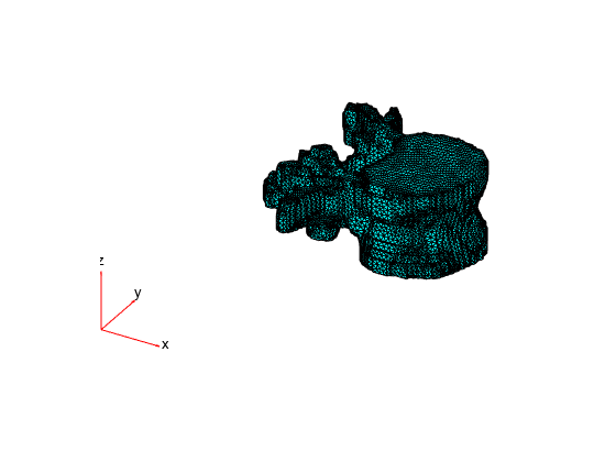
Generate the mesh from the model geometry. Specify the maximum edge length, and specify that the minimum edge length is half of the maximum edge length. The elements are quadratic tetrahedra.

msh = generateMesh(model,Hmax=hMax,Hmin=hMax/2);
pdemesh(model);

Assign Material Properties

Bone material properties vary based on spatial location and direction:

In this example, you assign spatially varying, transversely isotropic linear elastic material properties.

Extract HU Values Within Vertebra Mask

To assign spatially varying material properties, you need to map CT intensity values to FE mesh coordinates.

Load the original, unsegmented CT scan using a medicalVolume object. The medicalVolume object automatically converts the intensity to Hounsfield units (HU). The HU value is a standard for measuring radiodensity.

DCMData = medicalVolume(dataFolder);

Extract the indices and intensities of CT voxels inside the vertebra mask.

trueIdx = find(labelVol.Voxels==1);
HUVertebra = double(DCMData.Voxels(trueIdx));

Convert the linear indices in trueIdx into subscript indices, in units of voxels.

[row,col,slice] = ind2sub(size(labelVol.Voxels),trueIdx);

Transform the subscript indices into patient coordinates and convert the coordinates from millimeters to meters.

[X2,Y2,Z2] = intrinsicToWorld(R,col,row,slice);
HUVertebraMeters = [X2 Y2 Z2].*10^-3;

Map HU Values from CT Voxels to Mesh Nodes

The FE node coordinates are scattered and not aligned with the CT voxel grid. Create a scatteredInterpolant object to define the 3-D interpolation between the voxel grid and FE nodes.

F = scatteredInterpolant(HUVertebraMeters,HUVertebra);

Specify Coefficients

Specify the PDE coefficients for the model. In this structural analysis, the c coefficient defines the material stiffness of the model, which is inversely related to compliance. To define a spatially varying c coefficient in Partial Differential Equation Toolbox™, represent c in function form. In this example, the HU2TransverseIsotropy helper function defines transversely isotropic material properties based on bone density. Bone density is calculated for a given location using the scattered interpolant F. The helper function is wrapped in an anonymous function, ccoeffunc, which passes the location and state structures to HU2TransverseIsotropy. The FE solver automatically computes location and state structure arrays and passes them to your function during the simulation.

ccoeffunc = @(location,state) HU2TransverseIsotropy(location,state,F);
specifyCoefficients(model,'m',0, ...
    'd',0, ...
    'c',ccoeffunc, ...
    'a',0, ...
    'f',[0;0;0]);

Apply Loading and Solve Model

To simulate axial loading of the vertebra, fix the bottom surface and apply a downward load to the top surface. To simulate distributed loading, the load is applied as a pressure.

Identify the faces in the model geometry to apply the boundary conditions. In this example, the faces were identified using visual inspection of the plot created above using pdegplot.

bottomSurfaceFace = 1;
topSurfaceFace = 250;

Specify the total force to apply, in newtons.

forceInput = -3000;

Estimate the area of the top surface.

nf2=findNodes(model.Mesh,"region",Face=topSurfaceFace);
positions = model.Mesh.Nodes(:,nf2)';
surfaceShape = alphaShape(positions(:,1:2));
faceArea = area(surfaceShape);

Calculate the pressure magnitude as a function of force and area, in pascals.

inputPressure_Pa = forceInput/faceArea;

Apply the boundary conditions.

applyBoundaryCondition(model,"dirichlet",Face=bottomSurfaceFace,u=[0,0,0]);            
applyBoundaryCondition(model,"neumann",Face=topSurfaceFace,g=[0;0;inputPressure_Pa]);

Solve the model. The output is a StationaryResults (Partial Differential Equation Toolbox) object that contains nodal displacements and their gradients.

Rs = solvepde(model);

Analyze Results

View the results of the simulation by plotting the axial displacement, stress, and strain within the model.

Displacement

Plot axial displacement, in millimeters, for the full model by using the pdeplot3D function.

Uz = Rs.NodalSolution(:,3)*10^3;
pdeplot3D(model,"ColorMapData",Uz)
clim([-0.15 0])
title("Axial Displacement (mm)")

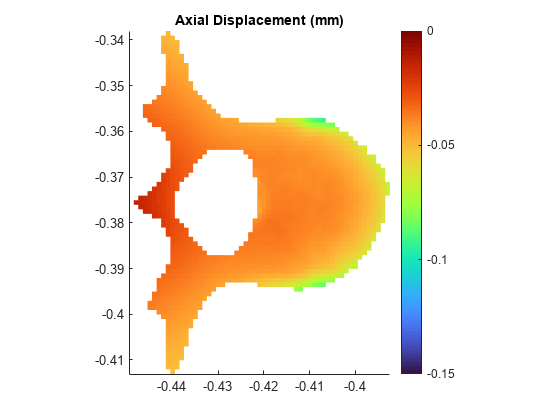
Plot displacement in a transverse slice at the midpoint of vertebral height.

Create a rectangular grid that covers the geometry of the transverse (xy) slice with spacing of 1 mm in each direction. The x and y vectors define the spatial limits and spacing in the transverse plane, and z is a scalar the provides the midpoint of vertebral height. The Xg, Yg, and Zg variables define the grid coordinates.

x = min(msh.Nodes(1,:)):0.001:max(msh.Nodes(1,:));
y = min(msh.Nodes(2,:)):0.001:max(msh.Nodes(2,:));
z = min(msh.Nodes(3,:))+0.5*(max(msh.Nodes(3,:))-min(msh.Nodes(3,:)));

[Xg,Yg] = meshgrid(x,y);
Zg = z*ones(size(Xg));

Interpolate normal axial displacement onto the grid coordinates by using the interpolateSolution (Partial Differential Equation Toolbox) object function. Convert displacement from meters to millimeters, and reshape the displacement vector to the grid size.

U = interpolateSolution(Rs,Xg,Yg,Zg,3);
U = U*10^3;
Ug = reshape(U,size(Xg));

Plot axial displacement in the transverse slice.

surf(Xg,Yg,Ug,LineStyle="none")
axis equal
grid off
view(0,90)
colormap("turbo")
colorbar
clim([-0.15 0])
title("Axial Displacement (mm)")

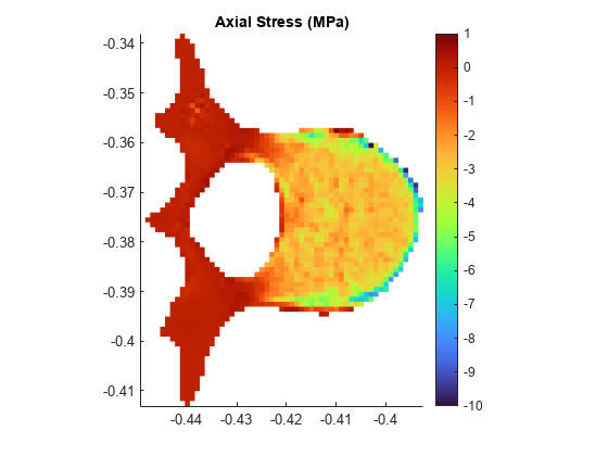
Stress

In a structural analysis, stress is the product of the c coefficient and the gradients of displacement. Calculate normal stresses at the transverse slice grid coordinates by using the evaluateCGradient (Partial Differential Equation Toolbox) object function.

[cgradx,cgrady,cgradz] = evaluateCGradient(Rs,Xg,Yg,Zg,3);

Convert normal axial stress to megapascals, and reshape the stress vector to the grid size.

cgradz = cgradz*10^-6;
cgradzg = reshape(cgradz,size(Xg));

Plot the normal axial stress in the transverse slice.

surf(Xg,Yg,cgradzg,LineStyle="none");
axis equal
grid off
view(0,90)
colormap("turbo")
colorbar
clim([-10 1])
title("Axial Stress (MPa)")

Strain

In a structural analysis, strain is the gradient of the displacement result. Extract the normal strain at the transverse slice grid coordinates by using the evaluateGradient (Partial Differential Equation Toolbox) object function.

[gradx,grady,gradz] = evaluateGradient(Rs,Xg,Yg,Zg,3);

Reshape the axial strain vector to the grid size.

gradzg = reshape(gradz,size(Xg));

Plot the axial strain in the transverse slice.

surf(Xg,Yg,gradzg,LineStyle="none");
axis equal
grid off
view(0,90)
colormap("turbo")
colorbar
clim([-0.008 0])
title("Axial Strain")

Helper Functions

The HU2TransverseIsotropy helper function specifies transverse isotropic material properties using these steps:

function ccoeff = HU2TransverseIsotropy(location,state,F)
    HU = F(location.x,location.y,location.z);
    rho = 5.2+0.8*HU;
    E3 = -34.7 + 3.230.*rho;
    E12 = 0.333*E3;
    v12 = 0.104;
    v3 = 0.381;
    G = 0.121*E3;

    ccoeff = zeros(45,length(location.x));
    for i = 1:length(location.x)
        cMatrix = elasticityTransOrthoC3D(E12(i),E3(i),v12,v3,G(i));
        nineMat = SixMat2NineMat(cMatrix);
        ccoeff(:,i) = SquareMat2CCoeffVec(nineMat);
    end
end

The elasticityTransOrthoC3D helper function defines the 6-by-6 compliance matrix for a transversely isotropic linear elastic material based on the elastic moduli, E12 and E3, bulk modulus, G, and Poisson's ratios, v12 and v3. The helper function converts all modulus values from megapascals to pascals before computing the compliance matrix.

function C = elasticityTransOrthoC3D(E12,E3,v12,v3,G)
    E12 = E12*10^6;
    E3 = E3*10^6;
    G = G*10^6;
    v_zp = (E3*v3)/E12;
    
    C = zeros(6,6);
    C(1,1) = 1/E12;
    C(1,2) = -v12/E12;
    C(1,3)= -v_zp/E3;
    C(2,1) = C(1,2);
    C(2,2) = 1/E12;
    C(2,3) = -v_zp/E3;
    C(3,1) = -v3/E12;
    C(3,2) = C(2,3);
    C(3,3) = 1/E3;
    C(4,4) = 1/(2*G);
    C(5,5) = 1/(2*G);
    C(6,6) = (1+v12)/E12;
    
    C=inv(C);

end

The SixMat2NineMat helper function converts a 6-by-6 c coefficient matrix in Voigt notation to a 9-by-9 matrix corresponding to expanded form.

function nineMat = SixMat2NineMat(sixMat)

    for i = 1:6
        nineVecs(i,:) = sixMat(i,[1 6 5 6 2 4 5 4 3]);
    end
    
    nineMat = [ nineVecs(1,:); ...
        nineVecs(6,:); ...
        nineVecs(5,:); ...
    
        nineVecs(6,:); ...
        nineVecs(2,:); ...
        nineVecs(4,:); ...
    
        nineVecs(5,:); ...
        nineVecs(4,:); ...
        nineVecs(3,:)];

end

The SquareMat2CCoeffVec converts a 9-by-9 c coefficient matrix into vector form as required by Partial Differential Equation Toolbox. This helper function creates a 45-element vector, corresponding to the "3N(3N+1)/2-Element Column Vector c, 3-D Systems" case in c Coefficient for specifyCoefficients (Partial Differential Equation Toolbox).

function c45Vec = SquareMat2CCoeffVec(nineMat)

    C11 = [nineMat(1,1) nineMat(1,2) nineMat(2,2) nineMat(1,3) nineMat(2,3) nineMat(3,3)];
    C12 = [nineMat(1,4) nineMat(2,4) nineMat(3,4) nineMat(1,5) nineMat(2,5) nineMat(3,5) ...
        nineMat(1,6) nineMat(2,6) nineMat(3,6)];
    C13 = [nineMat(1,7) nineMat(2,7) nineMat(3,7) nineMat(1,8) nineMat(2,8) nineMat(3,8) ...
        nineMat(1,9) nineMat(2,9) nineMat(3,9)];
    C22 = [nineMat(4,4) nineMat(4,5) nineMat(5,5) nineMat(4,6) nineMat(5,6) nineMat(6,6)];
    C23 = [nineMat(4,7) nineMat(5,7) nineMat(6,7) nineMat(4,8) nineMat(5,8) nineMat(6,8) ...
        nineMat(4,9) nineMat(5,9) nineMat(6,9)];
    C33 = [nineMat(7,7) nineMat(7,8) nineMat(8,8) nineMat(7,9) nineMat(8,9) nineMat(9,9)];
    c45Vec  = [C11 C12 C22 C13 C23 C33]';

end

References

[1] Turbucz, Mate, Agoston Jakab Pokorni, György Szőke, Zoltan Hoffer, Rita Maria Kiss, Aron Lazary, and Peter Endre Eltes. “Development and Validation of Two Intact Lumbar Spine Finite Element Models for In Silico Investigations: Comparison of the Bone Modelling Approaches.” Applied Sciences 12, no. 20 (January 2022): 10256. https://doi.org/10.3390/app122010256.

[2] Unnikrishnan, Ginu U., and Elise F. Morgan. “A New Material Mapping Procedure for Quantitative Computed Tomography-Based, Continuum Finite Element Analyses of the Vertebra.” Journal of Biomechanical Engineering 133, no. 7 (July 1, 2011): 071001. https://doi.org/10.1115/1.4004190.