Main Content

fir1

R2026b

Window-based FIR filter design

Description

b = fir1(n,Wn) uses a Hamming window to design a lowpass, bandpass, or multiband FIR filter with linear phase and order n. The filter type depends on the length of Wn. The function returns a row vector b containing n+1 coefficients.

example

b = fir1(n,Wn,ftype) designs a lowpass, highpass, bandpass, bandstop, or multiband filter, depending on the value of ftype and the number of elements of Wn.

example

b = fir1(___,window) designs the filter using the vector specified in window and any of the arguments from previous syntaxes.

example

b = fir1(___,scaleopt) additionally specifies whether or not the magnitude response of the filter is normalized.

Note:   Use fir2 for windowed filters with arbitrary frequency response.

Examples

collapse all

Design a 48th-order FIR bandpass filter with passband 0.35π≤ω≤0.65π rad/sample. Visualize its magnitude and phase responses.

b = fir1(48,[0.35 0.65]);
freqz(b,1,512)
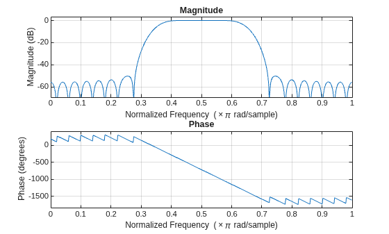
Figure contains 2 axes objects. Axes object 1 with title Phase, xlabel Normalized Frequency (\times\pi rad/sample), ylabel Phase (degrees) contains an object of type line. Axes object 2 with title Magnitude, xlabel Normalized Frequency (\times\pi rad/sample), ylabel Magnitude (dB) contains an object of type line.

Load chirp.mat. The file contains a signal, y, that has most of its power above Fs/4, or half the Nyquist frequency. The sample rate is 8192 Hz.

Design a 34th-order FIR highpass filter to attenuate the components of the signal below Fs/4. Use a cutoff frequency of 0.48 and a Chebyshev window with 30 dB of ripple.

load chirp

t = (0:length(y)-1)/Fs;

bhi = fir1(34,0.48,"high",chebwin(35,30));
freqz(bhi,1)
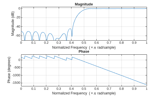
Figure contains 2 axes objects. Axes object 1 with title Phase, xlabel Normalized Frequency (\times\pi rad/sample), ylabel Phase (degrees) contains an object of type line. Axes object 2 with title Magnitude, xlabel Normalized Frequency (\times\pi rad/sample), ylabel Magnitude (dB) contains an object of type line.

Filter the signal. Display the original and highpass-filtered signals. Use the same y-axis scale for both plots.

outhi = filter(bhi,1,y);

tiledlayout("flow")
nexttile
plot(t,y)
title("Original Signal")
ys = ylim;

nexttile
plot(t,outhi)
title("Highpass Filtered Signal")
xlabel("Time (s)")
ylim(ys)
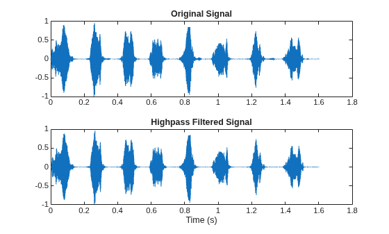
Figure contains 2 axes objects. Axes object 1 with title Original Signal contains an object of type line. Axes object 2 with title Highpass Filtered Signal, xlabel Time (s) contains an object of type line.

Design a lowpass filter with the same specifications. Filter the signal and compare the result to the original. Use the same y-axis scale for both plots.

blo = fir1(34,0.48,chebwin(35,30));

outlo = filter(blo,1,y);

tiledlayout("flow")
nexttile
plot(t,y)
title("Original Signal")
ys = ylim;

nexttile
plot(t,outlo)
title("Lowpass Filtered Signal")
xlabel("Time (s)")
ylim(ys)
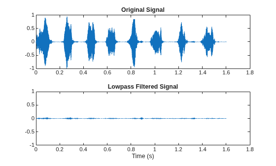
Figure contains 2 axes objects. Axes object 1 with title Original Signal contains an object of type line. Axes object 2 with title Lowpass Filtered Signal, xlabel Time (s) contains an object of type line.

Design a 46th-order FIR filter that attenuates normalized frequencies below 0.4π rad/sample and between 0.6π and 0.9π rad/sample. Call it bM. Compute its frequency response.

ord = 46;

low = 0.4;
bnd = [0.6 0.9];

bM = fir1(ord,[low bnd]);
[hbM,f] = freqz(bM,1);

Redesign bM so that it passes the bands it was attenuating and stops the other frequencies. Call the new filter bW. Display the frequency responses of the filters.

bW = fir1(ord,[low bnd],"DC-1");

[hbW,~] = freqz(bW,1);
plot(f/pi,mag2db(abs(hbM)),f/pi,mag2db(abs(hbW)))
legend("bM","bW",Location="best")
ylim([-75 5])
grid
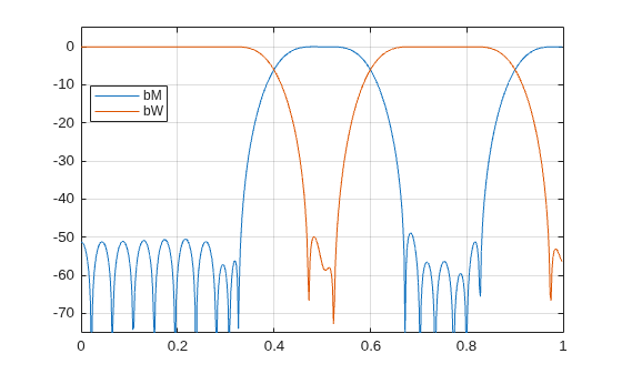
Figure contains an axes object. The axes object contains 2 objects of type line. These objects represent bM, bW.

Redesign bM using a Hann window. (The "DC-0" is optional.) Compare the magnitude responses of the Hamming and Hann designs.

hM = fir1(ord,[low bnd],"DC-0",hann(ord+1));

hhM = freqz(hM,1);
plot(f/pi,mag2db(abs(hbM)),f/pi,mag2db(abs(hhM)))
legend("Hamming","Hann",Location="northwest")
ylim([-75 5])
grid
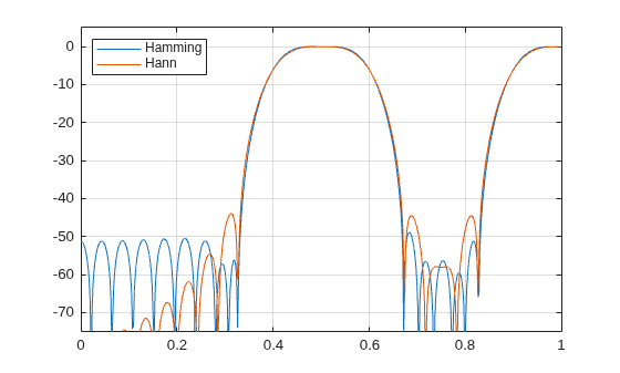
Figure contains an axes object. The axes object contains 2 objects of type line. These objects represent Hamming, Hann.

Redesign bW using a Tukey window. Compare the magnitude responses of the Hamming and Tukey designs.

tW = fir1(ord,[low bnd],"DC-1",tukeywin(ord+1));

htW = freqz(tW,1);
plot(f/pi,mag2db(abs(hbW)),f/pi,mag2db(abs(htW)))
legend("Hamming","Tukey",Location="best")
ylim([-75 5])
grid
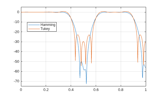
Figure contains an axes object. The axes object contains 2 objects of type line. These objects represent Hamming, Tukey.

Input Arguments

collapse all

Filter order, specified as a positive integer.

For highpass and bandstop configurations, fir1 uses an even filter order. The order must be even because odd-order symmetric FIR filters must have zero gain at the Nyquist frequency. If you specify an odd value of n for a highpass or bandstop filter, then fir1 increments n by 1.

When you specify this argument, fir1 returns b with n+1 coefficients, where n is the highest degree of the filter polynomial with coefficients b. If b contains trailing zero coefficients, the effective filter order can be lower than n. To determine the filter order of b, use filtord(b).

Data Types: double

Frequency constraints, specified as a scalar, a two-element vector, or a multi-element vector. All elements of Wn must be strictly greater than 0 and strictly smaller than 1, where 1 corresponds to the Nyquist frequency: 0 < Wn < 1. The Nyquist frequency is half the sample rate or π rad/sample.

  • If Wn is a scalar, then fir1 designs a lowpass or highpass filter with cutoff frequency Wn. The cutoff frequency is the frequency at which the normalized gain of the filter is –6 dB.

  • If Wn is the two-element vector [w1 w2], where w1 < w2, then fir1 designs a bandpass or bandstop filter with lower cutoff frequency w1 and higher cutoff frequency w2.

  • If Wn is the multi-element vector [w1 w2 ... wn], where w1 < w2 < … < wn, then fir1 returns an nth-order multiband filter with bands 0 < ω < w1, w1 < ω < w2,  …, wn < ω < 1.

Data Types: double

Filter type, specified as one of the following:

  • "low" specifies a lowpass filter with cutoff frequency Wn. "low" is the default for scalar Wn.

  • "high" specifies a highpass filter with cutoff frequency Wn.

  • "bandpass" specifies a bandpass filter if Wn is a two-element vector. "bandpass" is the default when Wn has two elements.

  • "stop" specifies a bandstop filter if Wn is a two-element vector.

  • "DC-0" specifies that the first band of a multiband filter is a stopband. "DC-0" is the default when Wn has more than two elements.

  • "DC-1" specifies that the first band of a multiband filter is a passband.

Window, specified as a vector. The window vector must have n + 1 elements. If you do not specify window, then fir1 uses a Hamming window. For a list of available windows, see Windows.

fir1 does not automatically increase the length of window if you attempt to design a highpass or bandstop filter of odd order.

Example: kaiser(n+1,0.5) specifies a Kaiser window with shape parameter 0.5 to use with a filter of order n.

Example: hamming(n+1) is equivalent to leaving the window unspecified.

Data Types: double

Normalization option, specified as either "scale" or "noscale".

  • "scale" normalizes the coefficients so that the magnitude response of the filter at the center of the passband is 1 (0 dB).

  • "noscale" does not normalize the coefficients.

Output Arguments

collapse all

Filter coefficients, returned as a row vector of length n + 1. The coefficients are sorted in descending powers of the Z-transform variable z:

B(z) = b(1) + b(2)z–1 + … + b(n+1)z–n.

Algorithms

fir1 uses a least-squares approximation to compute the filter coefficients and then smooths the impulse response with window.

References

[1] Digital Signal Processing Committee of the IEEE Acoustics, Speech, and Signal Processing Society, eds. Programs for Digital Signal Processing. New York: IEEE Press, 1979, Algorithm 5.2.

Extended Capabilities

expand all

C/C++ Code Generation
Generate C and C++ code using MATLAB® Coder™.

GPU Code Generation
Generate CUDA® code for NVIDIA® GPUs using GPU Coder™.

Version History

Introduced before R2006a

expand all