stepz

Step response of digital filter

collapse all in page

Syntax

[h,t] = stepz(b,a)

[h,t] = stepz(B,A,"ctf")

[h,t] = stepz({B,A,g},"ctf")

[h,t] = stepz(d)

[h,t] = stepz(sos)

[h,t] = stepz(___,n)

[h,t] = stepz(___,n,fs)

stepz(___)

Description

[h,t] = stepz(b,a) returns the step response of the specified digital filter. Specify a digital filter with numerator coefficients b and denominator coefficients a. The function returns the step response vector in h and the sample times in t.

example

[h,t] = stepz(B,A,"ctf") returns the step response of the digital filter represented as Cascaded Transfer Functions (CTF) with numerator coefficients B and denominator coefficients A. (since R2024b)

example

[h,t] = stepz({B,A,g},"ctf") returns the step response of the digital filter in CTF format. Specify the filter with numerator coefficients B, denominator coefficients A, and scaling values g across filter sections. (since R2024b)

example

[h,t] = stepz(d) returns the step response for the digital filter d.

[h,t] = stepz(sos) returns the step response corresponding to the second-order sections matrix sos.

[h,t] = stepz(___,n) computes the first n samples of the step response. This syntax can include any combination of input arguments from the previous syntaxes.

[h,t] = stepz(___,n,fs) computes n samples and produces a vector t so that the samples are spaced 1/fs units apart.

stepz(___) with no output arguments plots the step response of the filter.

example

Examples

collapse all

Step Response of a Butterworth Filter

Open Live Script

Create a third-order Butterworth filter with normalized half-power frequency $0.4 π$ rad/sample. Display its step response.

[b,a] = butter(3,0.4);
stepz(b,a)

Figure contains an axes object. The axes object with title Step Response, xlabel n (samples), ylabel Amplitude contains an object of type stem.

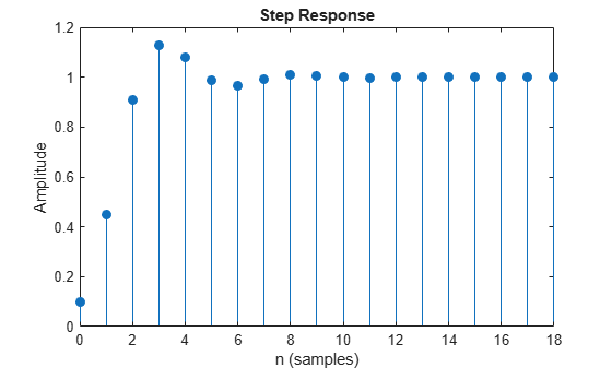
Create an identical filter using designfilt and display its step response.

d = designfilt('lowpassiir','FilterOrder',3,'HalfPowerFrequency',0.4);
stepz(d)

Figure contains an axes object. The axes object with title Step Response, xlabel n (samples), ylabel Amplitude contains an object of type stem.

Step Response of an Elliptic Filter

Open Live Script

Design a fourth-order lowpass elliptic filter with normalized passband frequency $0.4 π$ rad/sample. Specify a passband ripple of 0.5 dB and a stopband attenuation of 20 dB. Plot the first 50 samples of the filter's step response.

[b,a] = ellip(4,0.5,20,0.4);
stepz(b,a,50)

Figure contains an axes object. The axes object with title Step Response, xlabel n (samples), ylabel Amplitude contains an object of type stem.

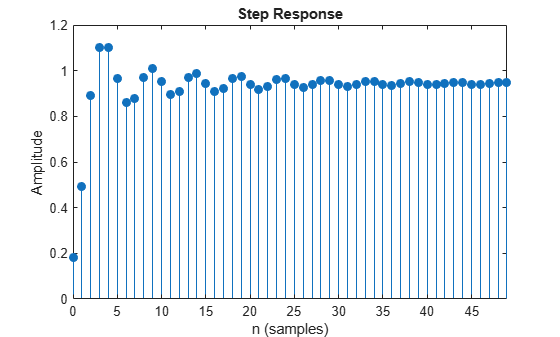
Create the same filter using designfilt and display its step response.

d = designfilt('lowpassiir','FilterOrder',4,'PassbandFrequency',0.4, ...
               'PassbandRipple',0.5,'StopbandAttenuation',20, ...
               'DesignMethod','ellip');
stepz(d,50)

Figure contains an axes object. The axes object with title Step Response, xlabel n (samples), ylabel Amplitude contains an object of type stem.

Step Response from Cascaded Transfer Functions

Since R2024b

Open Live Script

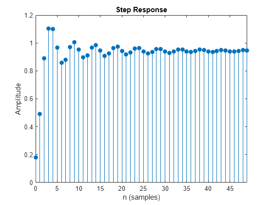
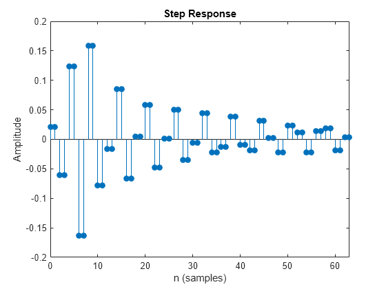
Design a 40th-order lowpass Chebyshev type II digital filter with a stopband edge frequency of 0.4 and stopband attenuation of 50 dB. Plot the first 64 samples of the filter step response using the filter coefficients in the CTF format.

[B,A] = cheby2(40,50,0.4,"ctf");

stepz(B,A,"ctf",64)

Figure contains an axes object. The axes object with title Step Response, xlabel n (samples), ylabel Amplitude contains an object of type stem.

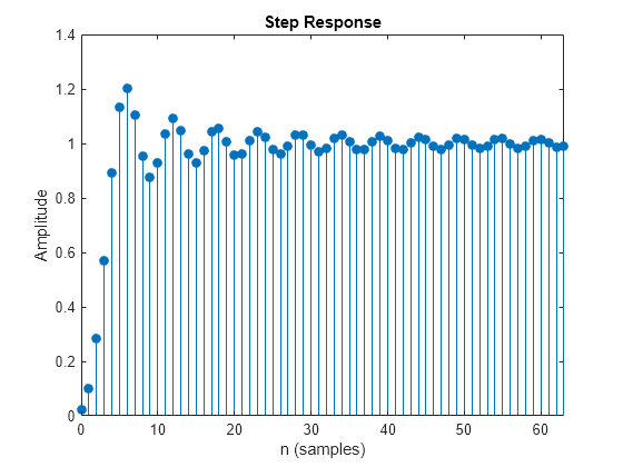
Design a 30th-order bandpass elliptic digital filter with passband edge frequencies of 0.3 and 0.7, passband ripple of 0.1 dB, and stopband attenuation of 50 dB. Plot the first 64 samples of the filter step response using the filter coefficients and gain in the CTF format.

[B,A,g] = ellip(30,0.1,50,[0.3 0.7],"ctf");
stepz({B,A,g},"ctf",64)

Figure contains an axes object. The axes object with title Step Response, xlabel n (samples), ylabel Amplitude contains an object of type stem.

Input Arguments

collapse all

`b`, `a` — Transfer function coefficients
vectors

Transfer function coefficients, specified as vectors. Express the transfer function in terms of b and a as

$H (z) = \frac{B (z)}{A (z)} = \frac{b_{1} + b_{2} z^{- 1} \dots + b_{n} z^{- (n - 1)} + b_{n + 1} z^{- n}}{a_{1} + a_{2} z^{- 1} \dots + a_{m} z^{- (m - 1)} + a_{m + 1} z^{- m}}$

Example: b = [1 3 3 1]/6 and a = [3 0 1 0]/3 specify a third-order Butterworth filter with normalized 3 dB frequency 0.5π rad/sample.

Data Types: double | single
Complex Number Support: Yes

`B,A` — Cascaded transfer function (CTF) coefficients
scalars | vectors | matrices

Since R2024b

Cascaded transfer function (CTF) coefficients, specified as scalars, vectors, or matrices. B and A list the numerator and denominator coefficients of the cascaded transfer function, respectively.

B must be of size L-by-(m + 1) and A must be of size L-by-(n + 1), where:

L represents the number of filter sections.
m represents the order of the filter numerators.
n represents the order of the filter denominators.

For more information about the cascaded transfer function format and coefficient matrices, see Specify Digital Filters in CTF Format.

Note

If any element of A(:,1) is not equal to 1, then stepz normalizes the filter coefficients by A(:,1). In this case, A(:,1) must be nonzero.

Data Types: double | single
Complex Number Support: Yes

`g` — Scale values
scalar | vector

Since R2024b

Scale values, specified as a real-valued scalar or as a real-valued vector with L + 1 elements, where L is the number of CTF sections. The scale values represent the distribution of the filter gain across sections of the cascaded filter representation.

The stepz function applies a gain to the filter sections using the scaleFilterSections function depending on how you specify g:

Scalar — The function distributes the gain uniformly across all filter sections.
Vector — The function applies the first L gain values to the corresponding filter sections and distributes the last gain value uniformly across all filter sections.

Data Types: double | single

`d` — Digital filter
`digitalFilter` object

Digital filter, specified as a digitalFilter object. Use designfilt to generate a digital filter based on frequency-response specifications.

Example: d = designfilt('lowpassiir','FilterOrder',3,'HalfPowerFrequency',0.5) specifies a third-order Butterworth filter with normalized 3 dB frequency 0.5π rad/sample.

`sos` — Second-order section coefficients
matrix

Second-order section coefficients, specified as a matrix. sos is a K-by-6 matrix, where the number of sections, K, must be greater than or equal to 2. If the number of sections is less than 2, the function treats the input as a numerator vector. Each row of sos corresponds to the coefficients of a second-order (biquad) filter. The ith row of sos corresponds to [bi(1) bi(2) bi(3) ai(1) ai(2) ai(3)].

Example: s = [2 4 2 6 0 2;3 3 0 6 0 0] specifies a third-order Butterworth filter with normalized 3 dB frequency 0.5π rad/sample.

Data Types: double | single
Complex Number Support: Yes

`n` — Number of points over which to evaluate response
positive integer scalar | positive integer vector

Number of points over which to evaluate response, specified as a positive integer scalar or positive integer vector. If n is a positive integer scalar (t = [0:n-1]'), the function computes the first n samples of the step response. If n is a vector of integers, the step response is computed only at those integer values, with 0 denoting the time origin.

Data Types: double

`fs` — Sample rate
positive scalar

Sample rate, specified as a positive scalar. When the unit of time is seconds, fs is expressed in hertz.

Data Types: double

Output Arguments

collapse all

`h` — Step response
column vector

Step response, returned as a column vector. If the input to stepz is single precision, the function computes the step response using single-precision arithmetic. The output h is single precision.

`t` — Sample times
vector

Sample times, returned as a vector.

More About

collapse all

Cascaded Transfer Functions

Partitioning an IIR digital filter into cascaded sections improves its numerical stability and reduces its susceptibility to coefficient quantization errors. The cascaded form of a transfer function H(z) in terms of the L transfer functions H₁(z), H₂(z), …, H_L(z) is

$H (z) = \prod_{l = 1}^{L} H_{l} (z) = H_{1} (z) \times H_{2} (z) \times \dots \times H_{L} (z) .$

Specify Digital Filters in CTF Format

You can specify digital filters in the CTF format for analysis, visualization, and signal filtering. Specify a filter by listing its coefficients B and A. You can also include the filter scaling gain across sections by specifying a scalar or vector g.

Filter Coefficients

When you specify the coefficients as L-row matrices,

$B = [\begin{matrix} b_{11} & b_{12} & \dots & b_{1, m + 1} \\ b_{21} & b_{22} & \dots & b_{2, m + 1} \\ ⋮ & ⋮ & ⋱ & ⋮ \\ b_{L 1} & b_{L 2} & \dots & b_{L, m + 1} \end{matrix}], A = [\begin{matrix} a_{11} & a_{12} & \dots & a_{1, n + 1} \\ a_{21} & a_{22} & \dots & a_{2, n + 1} \\ ⋮ & ⋮ & ⋱ & ⋮ \\ a_{L 1} & a_{L 2} & \dots & a_{L, n + 1} \end{matrix}],$

it is assumed that you have specified the filter as a sequence of L cascaded transfer functions, such that the full transfer function of the filter is

$H (z) = \frac{b_{11} + b_{12} z^{- 1} + \dots + b_{1, m + 1} z^{- m}}{a_{11} + a_{12} z^{- 1} + \dots + a_{1, n + 1} z^{- n}} \times \frac{b_{21} + b_{22} z^{- 1} + \dots + b_{2, m + 1} z^{- m}}{a_{21} + a_{22} z^{- 1} + \dots + a_{2, n + 1} z^{- n}} \times \dots \times \frac{b_{L 1} + b_{L 2} z^{- 1} + \dots + b_{L, m + 1} z^{- m}}{a_{L 1} + a_{L 2} z^{- 1} + \dots + a_{L, n + 1} z^{- n}},$

where m ≥ 0 is the numerator order of the filter and n ≥ 0 is the denominator order.

If you specify both B and A as vectors, it is assumed that the underlying system is a one-section IIR filter (L = 1), with B representing the numerator of the transfer function and A representing its denominator.
If B is scalar, it is assumed that the filter is a cascade of all-pole IIR filters with each section having an overall system gain equal to B.
If A is scalar, it is assumed that the filter is a cascade of FIR filters with each section having an overall system gain equal to 1/A.

Note

To convert second-order section matrices to cascaded transfer functions, use the sos2ctf function.
To convert a zero-pole-gain filter representation to cascaded transfer functions, use the zp2ctf function.

Coefficients and Gain

If you have an overall scaling gain or multiple scaling gains factored out from the coefficient values, you can specify the coefficients and gain as a cell array of the form {B,A,g}. Scaling filter sections is especially important when you work with fixed-point arithmetic to ensure that the output of each filter section has similar amplitude levels, which helps avoid inaccuracies in the filter response due to limited numeric precision.

The gain can be a scalar overall gain or a vector of section gains.

If the gain is scalar, the value applies uniformly to all the cascade filter sections.
If the gain is a vector, it must have one more element than the number of filter sections L in the cascade. Each of the first L scale values applies to the corresponding filter section, and the last value applies uniformly to all the cascade filter sections.

If you specify the coefficient matrices and gain vector as

it is assumed that the transfer function of the filter system is

$H (z) = g_{S} (g_{1} \frac{b_{11} + b_{12} z^{- 1} + \dots + b_{1, m + 1} z^{- m}}{a_{11} + a_{12} z^{- 1} + \dots + a_{1, n + 1} z^{- n}} \times g_{2} \frac{b_{21} + b_{22} z^{- 1} + \dots + b_{2, m + 1} z^{- m}}{a_{21} + a_{22} z^{- 1} + \dots + a_{2, n + 1} z^{- n}} \times \dots \times g_{L} \frac{b_{L 1} + b_{L 2} z^{- 1} + \dots + b_{L, m + 1} z^{- m}}{a_{L 1} + a_{L 2} z^{- 1} + \dots + a_{L, n + 1} z^{- n}}) .$

Tips

You can obtain filters in CTF format, including the scaling gain. Use the outputs of digital IIR filter design functions, such as butter, cheby1, cheby2, and ellip. Specify the "ctf" filter-type argument in these functions and specify to return B, A, and g to get the scale values. (since R2024b)

Algorithms

stepz filters a length n step sequence using

filter(b,a,ones(1,n))

and plots the results using stem.

To compute n in the auto-length case, stepz either uses n = length(b) for the FIR case, or first finds the poles using p = roots(a) if length(a) is greater than 1.

If the filter is unstable, n is chosen to be the point at which the term from the largest pole reaches 10⁶ times its original value.

If the filter is stable, n is chosen to be the point at which the term due to the largest amplitude pole is 5 × 10^–5 of its original amplitude.

If the filter is oscillatory (poles on the unit circle only), stepz computes five periods of the slowest oscillation.

If the filter has both oscillatory and damped terms, n is chosen to equal five periods of the slowest oscillation or the point at which the term due to the pole of largest nonunit amplitude is 5 × 10^–5 times its original amplitude, whichever is greater.

stepz also allows for delays in the numerator polynomial. The number of delays is incorporated into the computation for the number of samples.

References

[1] Lyons, Richard G. Understanding Digital Signal Processing. Upper Saddle River, NJ: Prentice Hall, 2004.

Extended Capabilities

C/C++ Code Generation
Generate C and C++ code using MATLAB® Coder™.

Usage notes and limitations:

If the first input to stepz is a variable-size matrix at compile time, then it must not become a vector at runtime.

Version History

Introduced before R2006a

expand all

R2024b: Analyze filters using cascaded transfer functions

The stepz function supports inputs in the cascaded transfer function (CTF) format.

stepz

Syntax

Description

Examples

Step Response of a Butterworth Filter

Step Response of an Elliptic Filter

Step Response from Cascaded Transfer Functions

Input Arguments

`b`, `a` — Transfer function coefficients
vectors

`B,A` — Cascaded transfer function (CTF) coefficients
scalars | vectors | matrices

`g` — Scale values
scalar | vector

`d` — Digital filter
`digitalFilter` object

`sos` — Second-order section coefficients
matrix

`n` — Number of points over which to evaluate response
positive integer scalar | positive integer vector

`fs` — Sample rate
positive scalar

Output Arguments

`h` — Step response
column vector

`t` — Sample times
vector

More About

Cascaded Transfer Functions

Specify Digital Filters in CTF Format

Tips

Algorithms

References

Extended Capabilities

C/C++ Code Generation
Generate C and C++ code using MATLAB® Coder™.

Version History

R2024b: Analyze filters using cascaded transfer functions

See Also

Apps

Functions

stepz

Syntax

Description

Examples

Step Response of a Butterworth Filter

Step Response of an Elliptic Filter

Step Response from Cascaded Transfer Functions

Input Arguments

b, a — Transfer function coefficients vectors

B,A — Cascaded transfer function (CTF) coefficients scalars | vectors | matrices

g — Scale values scalar | vector

d — Digital filter digitalFilter object

sos — Second-order section coefficients matrix

n — Number of points over which to evaluate response positive integer scalar | positive integer vector

fs — Sample rate positive scalar

Output Arguments

h — Step response column vector

t — Sample times vector

More About

Cascaded Transfer Functions

Specify Digital Filters in CTF Format

Tips

Algorithms

References

Extended Capabilities

C/C++ Code Generation Generate C and C++ code using MATLAB® Coder™.

Version History

R2024b: Analyze filters using cascaded transfer functions

See Also

Apps

Functions

WeChat

`b`, `a` — Transfer function coefficients
vectors

`B,A` — Cascaded transfer function (CTF) coefficients
scalars | vectors | matrices

`g` — Scale values
scalar | vector

`d` — Digital filter
`digitalFilter` object

`sos` — Second-order section coefficients
matrix

`n` — Number of points over which to evaluate response
positive integer scalar | positive integer vector

`fs` — Sample rate
positive scalar

`h` — Step response
column vector

`t` — Sample times
vector

C/C++ Code Generation
Generate C and C++ code using MATLAB® Coder™.