Model
Reference another model to create model hierarchy
Libraries:
Simulink /
Ports & Subsystems
HDL Coder /
Ports & Subsystems
Description
The Model block references the specified model. It displays input and output ports that correspond to the top-level input and output ports of the referenced model. These ports allow you to connect the referenced model to other blocks in the parent model.
To determine whether the Model block is better suited for your goal than another block with similar functionality, see Explore Types of Simulink Components and Compare Capabilities of Simulink Components.
For instructions on how to reference a model with a Model block, see Reference Existing Models.
By default, the Model block displays a representation of the contents of the referenced model. For more information, see Preview Content of Model Components. To see the contents of a referenced model, double-click the Model block.
If you have a Simulink® Coder™ license, you can conceal the implementation details of a referenced model by protecting the model. To protect a model, see Protect Models to Conceal Contents (Simulink Coder). To reference a protected model, see Reference Protected Models from Third Parties.
Examples
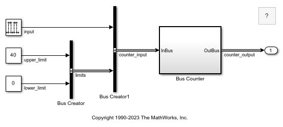
You can include one model in another by using a Model block. Each Model block is a model reference, or a reference to another model. You can reference a model multiple times without making redundant copies, and multiple models can reference the same model.
Open the example, which contains a model named BasicCounterAlgorithm.
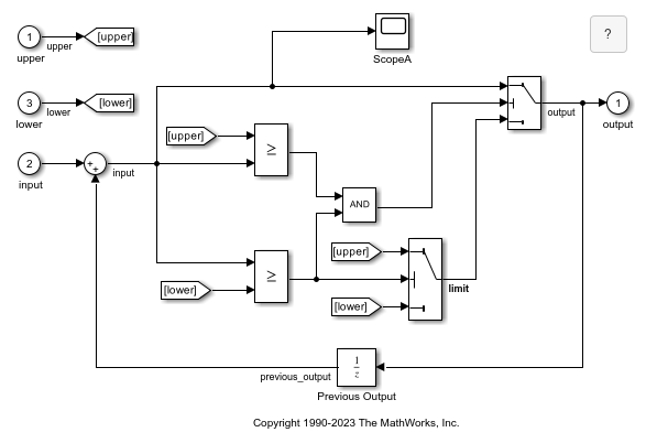
Before you reference a model, consider its configuration, interface, and contents.
The model named BasicCounterAlgorithm represents a counter algorithm and uses a fixed-step discrete solver.
To view the model interface, in the Simulink Toolstrip, on the Modeling tab, in the Design gallery, select Interface View. The Component Interface View opens.
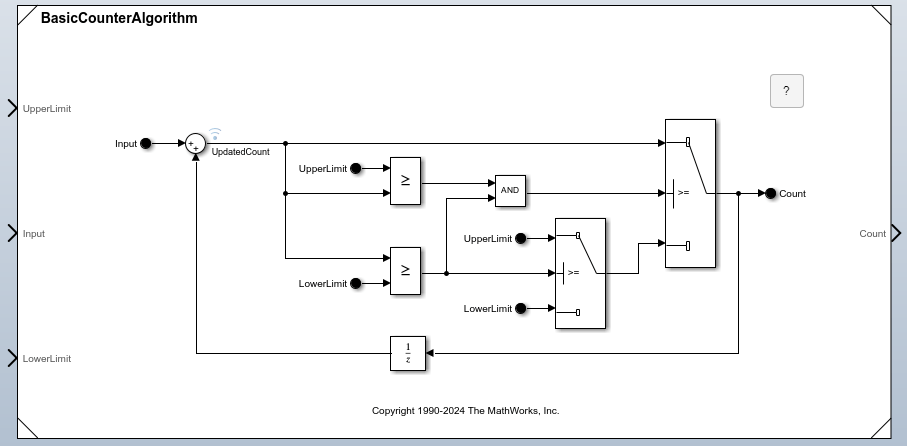
The model has three input ports and one output port.
The input port named
UpperLimitprovides the upper limit for the counter.The input port named
LowerLimitprovides the lower limit, or starting value, for the counter.The input port named
Inputprovides the value that the counter increments at each time step.The output port named
Countprovides the current count.
In a new model, add a Model block.

In the Property Inspector, set Model name to BasicCounterAlgorithm.

To better display the information on the block icon, drag a corner of the Model block until no information overlaps.

The Model block icon displays:
The name of the referenced model:
BasicCounterAlgorithmInput ports named
UpperLimit,Input, andLowerLimitAn output port named
Count
Configure the top model for fixed-step discrete simulation.
In the Simulink Toolstrip, on the Modeling tab, click Model Settings.
In the Configuration Parameters dialog box, on the Solver pane, set Type to
Fixed-stepand Solver todiscrete (no continuous states).Click OK.
Connect inputs and outputs to the Model block that match the expected inputs and outputs of the referenced model.
To represent the upper limit of the counter, add a Constant block with Constant value set to
100. Then, connect the block to the UpperLimit port.To represent the counter increment, add a Constant block with Constant value set to
1. Then, connect the block to the Input port.To represent the lower limit of the counter, add a Constant block with Constant value set to
0. Then, connect the block to the LowerLimit port.To display the counter output in a plot, add a Scope block. Then, connect the block to the Count port.

In the Simulink Toolstrip, on the Modeling tab, click Run.

The top model simulates and executes the referenced model. The Scope window shows the output count for the simulation.
Open the model SecondOrderSystemTop. The model contains a Ramp block that provides the input signal for a Model block that references a model of a second-order system. The Model block output signal connects to an Outport block.
topmdl = "SecondOrderSystemTop";
open_system(topmdl)
To navigate inside the referenced model, double-click the Model block. Alternatively, create a Simulink.BlockPath object for the Model block and use the open function to open the referenced model in the context of the model hierarchy.
mdlblkpath = Simulink.BlockPath(topmdl + "/Model");
open(mdlblkpath)
The referenced model implements the second-order system using a Transfer Fcn block and contains a Step block that models a change or disturbance to the system.
The system transfer function is specified in the Transfer Fcn block using two model workspace variables, wn and z, which represent the natural frequency of the system, in radians per second, and the system damping coefficient.
Configure the system with a natural frequency of 100 radians per second by specifying the value of the variable wn as 100 in the model workspace.
refmdl = "SecondOrderSystem";
mdlwksp = get_param(refmdl,"ModelWorkspace");
assignin(mdlwksp,"wn",100)
Configure the referenced model to use a local solver with a step size of 0.01 seconds. You can configure the settings for the referenced model from the top model using the Property Inspector or the Block Parameters dialog box.
Open the Property Inspector. On the Modeling tab, expand the Design section and select Property Inspector, or press Ctrl+Shift+I.
To open the Configuration Parameters dialog box for the referenced model, select the Model block. Then, in the Property Inspector, expand the Solver section and click the hyperlink next to the Use local solver parameter.
Configure the model to use a local solver when referenced in a model hierarchy. In the Configuration Parameters dialog box, on the Model Referencing pane, select Use local solver when referencing model.
Select the fixed-step
ode3as the local solver. On the Solver pane, from the Type list, selectFixed-step. Then, from the Solver list, selectode3 (Bogacki-Shampine).Set the local solver step size to 0.01 seconds. On the Solver pane, expand Solver details. Then, in the Fixed-step size (fundamental sample time) box, enter
0.01.Click OK.
Alternatively, use the set_param function to configure the parameters.
set_param(refmdl,UseModelRefSolver="on",...
    SolverType="Fixed-Step",Solver="ode3",FixedStep="0.01")
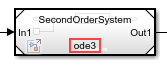
In the top model, the Model block indicates the local solver you specify.

Specify the communication step size for the model reference. The communication step size specifies when the parent and local solvers exchange data and is registered as a discrete sample time in the top model.
The Ramp block in the top model has a slope of 0.2, and the top solver uses a step size of 0.2 seconds. Because the input signal from the top model changes slowly compared to the dynamics of the second-order system, the communication step size can be much larger than the local solver step size without significant effect on the accuracy of the simulation results.
Specify the communication step size as 0.4 seconds. Select the Model block. Then, in the Property Inspector, under Solver, in the Communication step size box, enter 0.4.
Alternatively, use the set_param function to set the CommunicationStepSize parameter.
set_param(topmdl + "/Model",CommunicationStepSize="0.4")
Simulate the model, using the local solver to compute the response of the second-order system.
out = sim(topmdl);
To view the simulation results, open the Simulation Data Inspector. On the Simulation tab, under Review Results, click Data Inspector. Alternatively, call the Simulink.sdi.view function.
Simulink.sdi.view
Plot the signals named System Response and System Response - Top on separate subplots. Alternatively, use the Simulink.sdi.loadView function to load the view named FastSecondOrderSystem, which was created for this example.
Simulink.sdi.loadView("FastSecondOrderSystem.mldatx");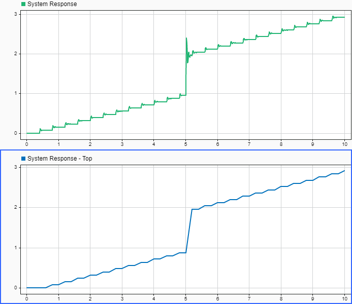
The System Response and System Response - Top signals are the same signal, logged in different locations. The System Response signal is logged inside the referenced model at a rate determined by the local solver step size. The System Response - Top signal is logged by the Outport block in the top model at a rate determined by the top solver step size. Because the local solver step size is much smaller than the top solver step size, the System Response signal captures the system response to the change in the input signal when the Step block output value changes with higher fidelity.
In the System Response signal, you can see the effect of the local solver interpolating the input signal with a zero-order hold between each communication step. If you zoom on the time axis around 5 seconds, you can see the oscillations in the system response to the step.

Open the model SecondOrderSystemTop. The model contains a Ramp block that provides the input signal for a Model block that references a model of a second-order system. The Model block output signal connects to an Outport block.
topmdl = "SecondOrderSystemTop";
open_system(topmdl)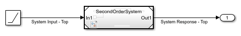
To navigate inside the referenced model, double-click the Model block. Alternatively, create a Simulink.BlockPath object for the Model block and use the open function to open the referenced model in the context of the model hierarchy.
mdlblkpath = Simulink.BlockPath(topmdl + "/Model");
open(mdlblkpath)
The referenced model implements the second-order system using a Transfer Fcn block and contains a Step block that models a change or disturbance to the system.
The system transfer function is specified in the Transfer Fcn block using two model workspace variables, wn and z, which represent the natural frequency of the system, in radians per second, and the system damping coefficient.
Configure the system with a natural frequency of 1 radian per second by specifying the value of the variable wn as 1 in the model workspace.
refmdl = "SecondOrderSystem";
mdlwksp = get_param(refmdl,"ModelWorkspace");
assignin(mdlwksp,"wn",1)
Configure the referenced model to use a local solver with a step size of 0.4 seconds. You can configure the settings for the referenced model from the top model using the Property Inspector or the Block Parameters dialog box.
Open the Property Inspector. On the Modeling tab, expand the Design section and select Property Inspector, or press Ctrl+Shift+I.
To open the Configuration Parameters dialog box for the referenced model, select the Model block. Then, in the Property Inspector, expand the Solver section and click the hyperlink next to the Use local solver parameter.
Configure the model to use a local solver when referenced in a model hierarchy. In the Configuration Parameters dialog box, on the Model Referencing pane, select Use local solver when referencing model.
Select the fixed-step
ode3as the local solver. On the Solver pane, from the Type list, selectFixed-step. Then, from the Solver list, selectode3 (Bogacki-Shampine).Set the local solver step size to 0.4 seconds. On the Solver pane, expand Solver details. Then, in the Fixed-step size (fundamental sample time) box, enter
0.4.Click OK.
Alternatively, use the set_param function to configure the parameters.
set_param(refmdl,UseModelRefSolver="on",...
    SolverType="Fixed-Step",Solver="ode3",FixedStep="0.4")
In the top model, the Model block indicates the local solver you specify.
When the local solver step size is larger than the parent solver step size, inherit the communication step size by specifying the Communication step size parameter as -1. The communication step size specifies when the parent solver and local solver exchange data and is registered as a discrete sample time in the parent model.
set_param(topmdl + "/Model",CommunicationStepSize="-1")
Simulate the model, using the local solver to compute the response of the second-order system.
out = sim(topmdl,StopTime="20");To view the simulation results, open the Simulation Data Inspector. On the Simulation tab, under Review Results, click Data Inspector. Alternatively, call the Simulink.sdi.view function.
Simulink.sdi.view
Plot the signals named System Response and System Response - Top on separate subplots. Alternatively, use the Simulink.sdi.loadView function to load the view named SlowSecondOrderSystem, which was created for this example.
Simulink.sdi.loadView("SlowSecondOrderSystem.mldatx");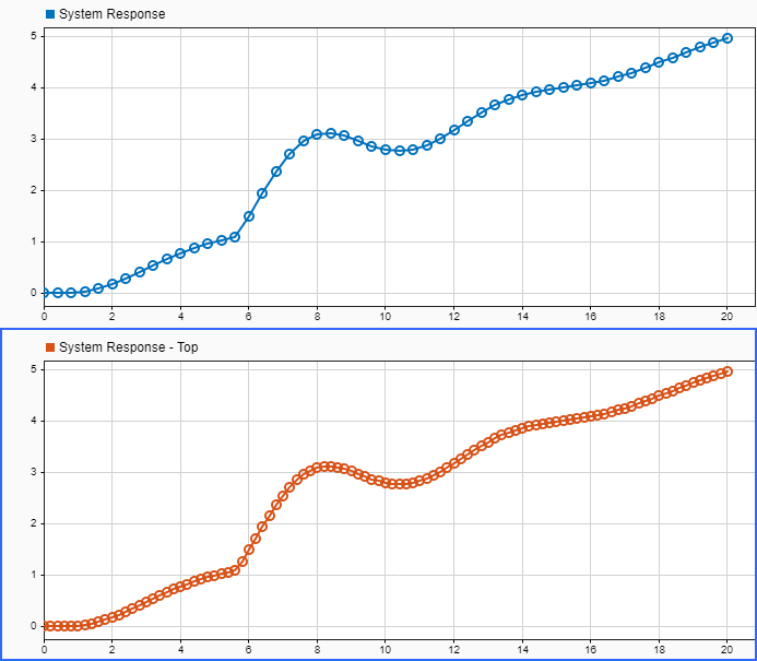
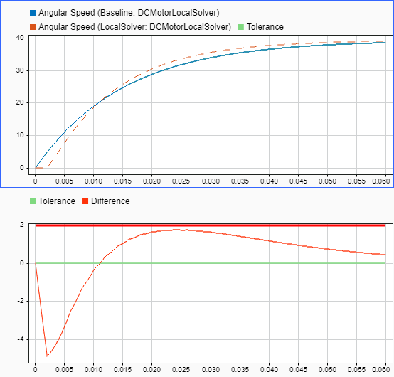
The System Response and System Response - Top signals are the same signal, logged in different locations. The System Response signal is logged inside the referenced model at a rate determined by the local solver step size. The System Response - Top signal is logged by the Outport block in the top model at a rate determined by the top solver step size. Fewer data points are logged for the System Response signal because the local solver step size is larger than the parent solver step size.
Extended Examples
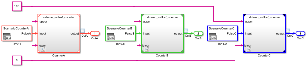
Component-Based Modeling with Model Reference
Walks you through simulation and code generation of a model that references another model multiple times.
Convert Subsystem to Referenced Model
Convert a subsystem to a referenced model by using the Model Reference Conversion Advisor or the Simulink.SubSystem.convertToModelReference function. For comprehensive instructions, see Convert Subsystems to Referenced Models.
Reuse Model Components from Files
Save components in separate subsystem and model files.
Improve Simulation Performance by Using Local Solvers
Improve simulation performance by using a local solver for a component with much faster dynamics compared to the rest of the system.
Ports
Input
Output
Control
Conditional Execution
The enable port appears at the top of the Model block. The port label is an icon that represents an enable signal.
The control signal that connects to the port determines when to execute the referenced model. For more information, see Conditionally Execute Referenced Models.
Dependencies
To enable this port, add an Enable block to the top level of the referenced model.
Data Types: single | double | int8 | int16 | int32 | int64 | uint8 | uint16 | uint32 | uint64 | Boolean | fixed point
The trigger port appears at the top of the Model block. The port label is an icon that represents a trigger signal.
The control signal that connects to the port determines when to execute the referenced model. For more information, see Conditionally Execute Referenced Models.
Dependencies
To enable this port, add a Trigger block to the
top level of the referenced model and set its Trigger
type to rising,
falling, or
either.
Data Types: single | double | int8 | int16 | int32 | int64 | uint8 | uint16 | uint32 | uint64 | Boolean | fixed point
The function-call port appears at the top of the Model block. The port label displays the name of the referenced model as a function.

The function-call control signal that connects to the port determines when to execute the referenced model. For more information, see Conditionally Execute Referenced Models.
Dependencies
To enable this port, add a Trigger block to the
top level of the referenced model and set its Trigger
type to
function-call.
Model Events Simulation
The initialize event port provides a function-call control signal that triggers a model initialize event, which initializes the states of the referenced model.
The referenced model can contain an Initialize Function block that corresponds to the model initialize event. For more information, see Using Initialize, Reinitialize, Reset, and Terminate Functions.
Dependencies
To enable this port, select Show model initialize port.
A reset event port provides a function-call control signal that triggers a model reset event, which resets the states of the referenced model.
The referenced model must contain a Reset Function block that corresponds to each model reset event. For more information, see Using Initialize, Reinitialize, Reset, and Terminate Functions.
To specify the port name, use the Event name parameter of the Event Listener block in the Reset Function block.
Dependencies
To enable this type of port, select Show model reset ports.
A reinitialize event port provides a function-call control signal that triggers a model reinitialize event, which reinitializes the states of the referenced model.
The referenced model must contain a Reinitialize Function block that corresponds to each model reinitialize event. For more information, see Using Initialize, Reinitialize, Reset, and Terminate Functions.
To specify the port name, use the Event name parameter of the Event Listener block in the Reinitialize Function block.
Dependencies
To enable this type of port, select Show model reinitialize ports.
The terminate event port provides a function-call control signal that triggers a model terminate event, which reads and saves the states of the referenced model.
The referenced model can contain a Terminate Function block that corresponds to the model terminate event. For more information, see Using Initialize, Reinitialize, Reset, and Terminate Functions.
Dependencies
To enable this port, select Show model terminate port.
Periodic event ports provide function-call control signals that specify when to execute the model. For an example, see Test Rate-Based Model Simulation Using Function-Call Generators.
Each port label displays information about the periodic event, such as the sample time of the corresponding Inport block. For example, the Model block in this image displays periodic event ports and references a model with two discrete rates: 0.01 and 0.1.
![A Model block has ports labeled D1[0.01] and D2[0.1].](model-block-periodic-event-ports.png)
Dependencies
To enable this type of port, set Schedule rates with to
Ports.
Parameters
Block Characteristics
Tips
To programmatically determine whether a Model block references a
protected model, use the get_param function to query the
read-only ProtectedModel parameter of the Model block.
If the referenced model is protected, the function returns "on". If
the referenced model is unprotected, the function returns
"off".
Extended Capabilities
Version History
Introduced before R2006aSee Also
Blocks
Functions
find_mdlrefs|depview|Simulink.VariantUtils.convertToVariantSubsystem|Simulink.SubSystem.convertToModelReference
Objects
Topics
- Compare Capabilities of Simulink Components
- Model Reference Behavior and Capabilities
- Reference Existing Models
- Configure Instance-Specific Values for Block Parameters in a Referenced Model
- Choose Simulation Modes for Model Hierarchies
- Protect Models to Conceal Contents (Simulink Coder)
- Use Local Solvers in Referenced Models