Detect Defects on Printed Circuit Boards Using YOLOX Network
R2026bThis example shows how to detect, localize, and classify defects in printed circuit boards (PCBs) using a YOLOX object detector.
PCBs contain individual electronic devices and their connections. Defects in PCBs can result in poor performance or product failures. By detecting defects in PCBs, production lines can remove faulty PCBs and ensure that electronic devices are of high quality.
Download Pretrained YOLOX Detector
By default, this example downloads a pretrained version of the YOLOX object detector [1] using the downloadTrainedNetwork helper function. The helper function is attached to this example as a supporting file. You can use the pretrained network to run the entire example without waiting for training to complete.
trainedPCBDefectDetectorNet_url = "https://ssd.mathworks.com/supportfiles/"+ ...
    "vision/data/trainedPCBDefectDetectorYOLOX.zip";
downloadTrainedNetwork(trainedPCBDefectDetectorNet_url,pwd);
Downloading pretrained network.
This can take several minutes to download...
Done.
load("trainedPCBDefectDetectorYOLOX.mat");Download PCB Defect Data Set
This example uses the PCB defect data set [2] [3]. The data set contains 1,386 images of PCB elements with synthesized defects. The data has six types of defect: missing hole, mouse bite, open circuit, short, spur, and spurious copper. Each image contains multiple defects of the same category in different locations. The data set contains bounding box and coordinate information for every defect in every image. The size of the data set is 1.87 GB.
Specify dataDir as the location of the data set. Download the data set using the downloadPCBDefectData helper function. This function is attached to the example as a supporting file.
dataDir = fullfile(tempdir,"PCBDefects");
downloadPCBDefectData(dataDir)
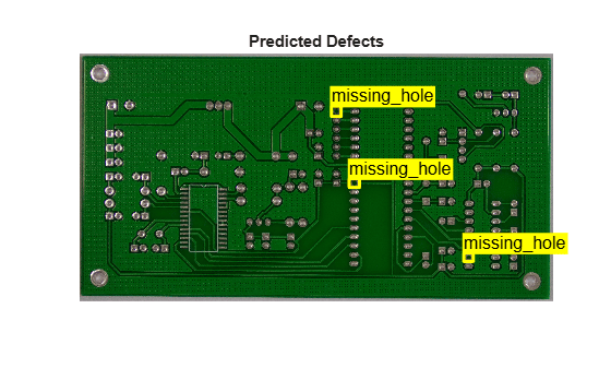
Perform Object Detection
Read a sample image from the data set.
sampleImage = imread(fullfile(dataDir,"PCB-DATASET-master","images", ...
    "Missing_hole","01_missing_hole_01.jpg"));
Predict the bounding boxes, labels, and class-specific confidence scores for each bounding box by using the detect function.
[bboxes,scores,labels] = detect(detector,sampleImage);
Display the results.
imshow(sampleImage)
showShape("rectangle",bboxes,Label=labels,Color="y");
title("Predicted Defects")
Prepare Data for Training
Create an image datastore that reads and manages the image data.
imageDir = fullfile(dataDir,"PCB-DATASET-master","images");
imds = imageDatastore(imageDir,FileExtensions=".jpg",IncludeSubfolders=true);
Create a file datastore that reads the annotation data from XML files. Specify a custom read function that parses the XML files and extracts the bounding box information. The custom read function, readPCBDefectAnnotations, is attached to the example as a supporting file.
annoDir = fullfile(dataDir,"PCB-DATASET-master","Annotations");
fds = fileDatastore(annoDir,ReadFcn=@readPCBDefectAnnotations, ...
    FileExtensions=".xml",IncludeSubfolders=true);
Save the labeled bounding box data as a box label datastore.
annotations = readall(fds);
tbl = struct2table(vertcat(annotations{:}));
blds = boxLabelDatastore(tbl);
Get the names of the object classes as a categorical vector.
classNames = categories(blds.LabelData{1,2})classNames = 6×1 cell array
"'missing_hole'"
"'mouse_bite'"
"'open_circuit'"
"'short'"
"'spur'"
"'spurious_copper'"
Combine the image and box label datastores.
ds = combine(imds,blds);
Analyze Object Class Distribution
Measure the distribution of class labels in the data set by using the countEachLabel function. The classes in this data set are balanced.
countEachLabel(blds)
ans = 6×3 table
       missing_hole    497    115
         mouse_bite    492    115
       open_circuit    482    116
              short    491    116
               spur    488    115
    spurious_copper    503    116
Partition Data
Prior to partitioning the data, set the global random state to the default state to ensure a higher reproducibility of results.
rng("default");Split the data set into training, validation, and test sets. Because the total number of images is relatively small, allocate a relatively large percentage (70%) of the data for training. Allocate 15% for validation and the rest for testing.
numImages = ds.numpartitions;
numTrain = floor(0.7*numImages);
numVal = floor(0.15*numImages);

shuffledIndices = randperm(numImages);
dsTrain = subset(ds,shuffledIndices(1:numTrain));
dsVal = subset(ds,shuffledIndices(numTrain+1:numTrain+numVal));
dsTest = subset(ds,shuffledIndices(numTrain+numVal+1:end));
Augment Training Data
Augment the training data by using the transform function with custom preprocessing operations specified by the augmentDataForPCBDefectDetection helper function. The helper function is attached to the example as a supporting file. The augmentDataForPCBDefectDetection function applies these augmentations to the input data:
Random horizontal flip (reflection)
Random resizing by a scale factor in the range [1, 1.1]
Random translation in the horizontal and vertical directions in the range [-50, 50] pixels
dsTrain = transform(dsTrain,@augmentDataForPCBDefectDetection);
Define YOLOX Object Detector Network Architecture
Create the YOLOX object detector by using the yoloxObjectDetector function. Specify the pretrained network created using CSP-DarkNet-53 as the base network and trained on the COCO data set [1]. Specify the class names and the network input size.
inputSize = [800 800 3];
detectorIn = yoloxObjectDetector("tiny-coco",classNames,InputSize=inputSize);
Specify Training Options
Specify network training options using the trainingOptions (Deep Learning Toolbox) function. Train the object detector using the SGDM solver for a maximum of 100 epochs. Specify the ValidationData name-value argument as the validation data. Set OutputNetwork to "best-validation-loss" to obtain the network with the lowest validation loss during training when the training finishes.
options = trainingOptions("sgdm", ...
    InitialLearnRate=5e-4, ...
    LearnRateSchedule="piecewise", ...
    LearnRateDropFactor=0.99, ...
    LearnRateDropPeriod=1, ...
    MiniBatchSize=20, ...
    MaxEpochs=100, ...
    ExecutionEnvironment="auto", ...
    Shuffle="every-epoch", ...
    VerboseFrequency=25, ...
    ValidationFrequency=100, ...
    ValidationData=dsVal, ...
    ResetInputNormalization=false, ...
    OutputNetwork="best-validation-loss", ...
    GradientThreshold=30, ...
    L2Regularization=5e-4);
Train Detector
To train the detector, set the doTraining variable to true. Train the detector by using the trainYOLOXObjectDetector function.
Train on one or more GPUs, if they are available. Using a GPU requires a Parallel Computing Toolbox™ license and a CUDA®-enabled NVIDIA® GPU. For more information, see GPU Computing Requirements (Parallel Computing Toolbox). Training takes about 7.5 hours on an NVIDIA Titan RTX™ with 24 GB of memory.
doTraining =false; if doTraining [detector,info] = trainYOLOXObjectDetector(dsTrain,detectorIn,options,"FreezeSubNetwork","none"); modelDateTime = string(datetime("now",Format="yyyy-MM-dd-HH-mm-ss")); save(fullfile(tempdir,"trainedPCBDefectDetectorYoloX"+modelDateTime+".mat"), ... "detector"); else load("trainedPCBDefectDetectorYOLOX.mat"); end
Evaluate Detector
Detect the bounding boxes for all test images. Set the detection threshold to a low value to detect as many objects as possible. This helps you evaluate the detection performance across a full range of detection score values.
detectionResults = detect(detector,dsTest,Threshold=0.01);
Calculate object detection metrics on the test set detection results by using the evaluateObjectDetection function.
metrics = evaluateObjectDetection(detectionResults,dsTest);
Calculate and display the average precision (AP) score for each class. Precision quantifies the ability of the detector to classify objects correctly.
AP = averagePrecision(metrics);
table(classNames,AP)
ans = 6×2 table
       'missing_hole'    0.9809
         'mouse_bite'    0.8571
       'open_circuit'    0.9432
              'short'    0.9735
               'spur'    0.9427
    'spurious_copper'    0.8899
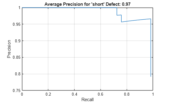
Calculate the recall and precision values for the detection of each defect object. Recall quantifies the ability of the detector to detect all relevant objects for a class. A precision-recall (PR) curve highlights how precise a detector is at varying levels of recall. The ideal precision is 1 at all recall levels. Plot the PR curve for the test data.
classNameStrings = metrics.ClassNames; class =classNameStrings(4); [precision, recall, ~] = precisionRecall(metrics,ClassName=class); plot(recall{:},precision{:}) title(sprintf("Average Precision for '" + class + "' Defect: " + "%.2f",averagePrecision(metrics,ClassName=class)), interpreter="none") xlabel("Recall") ylabel("Precision") grid on
Evaluate Object Size-based Detection Metrics
Investigate the impact of object size on detector performance with the metricsByArea function, which computes the object detection metrics for specific object size ranges. To evaluate size-based metrics, you can define the object size ranges based on a custom set of ranges. First, break the test image bounding box sizes into small, medium, and large object size categories according to percentile boundaries of the 33rd and 66th percentile of the test set object area distribution.
Plot the test set object size distribution, where the bounding box area defines the object size.
testSetObjects = dsTest.UnderlyingDatastores{2};
objectLabels = readall(testSetObjects);
boxes = objectLabels(:,1);
boxes = vertcat(boxes{:});
boxArea = prod(boxes(:,3:4),2);
histogram(boxArea)
title("Bounding Box Area Distribution")
xlabel("Box Area");
ylabel("Count")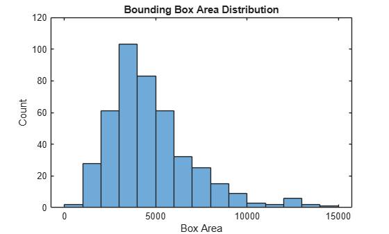
Define the bounding box area ranges, and then evaluate object detection metrics for the defined area ranges using metricsByArea. The mean average precision (mAP) metric of the trained detector performs approximately the same across small, medium, and large object sizes, with a slight performance improvement for medium objects.
boxPrctileBoundaries = prctile(boxArea,100*[1/3,2/3]);
metricsByArea(metrics,[0, boxPrctileBoundaries, inf])
ans = 3×4 table
             0    3.5737e+03    144    0.8416    0.8416
    3.5737e+03          5107    145    0.9605    0.9605
          5107           Inf    144    0.8854    0.8854
References
[1] Ge, Zheng, Songtao Liu, Feng Wang, Zeming Li, and Jian Sun. "YOLOX: Exceeding YOLO Series in 2021", arXiv, August 6, 2021. https://arxiv.org/abs/2107.08430.
[2] Huang, Weibo, and Peng Wei. "A PCB Dataset for Defects Detection and Classification." Preprint, submitted January 23, 2019. https://arxiv.org/abs/1901.08204.
[3] PCB-DATASET. Accessed December 20, 2022. https://github.com/Ironbrotherstyle/PCB-DATASET.
See Also
yoloxObjectDetector | trainYOLOXObjectDetector | detect | metricsByArea | evaluateObjectDetection | trainingOptions (Deep Learning Toolbox) | transform

