Image Processing Operator Approximation Using Deep Learning

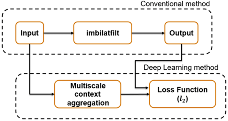
This example uses:

This example shows how to approximate an image filtering operation using a multiscale context aggregation network (CAN).

Operator approximation finds alternative ways to process images such that the result resembles the output from a conventional image processing operation or pipeline. The goal of operator approximation is often to reduce the time required to process an image.

Several classical and deep learning techniques have been proposed to perform operator approximation. Some classical techniques improve the efficiency of a single algorithm but cannot be generalized to other operations. Another common technique approximates a wide range of operations by applying the operator to a low resolution copy of an image, but the loss of high-frequency content limits the accuracy of the approximation.

Deep learning solutions enable the approximation of more general and complex operations. For example, the multiscale context aggregation network (CAN) presented by Q. Chen [1] can approximate multiscale tone mapping, photographic style transfer, nonlocal dehazing, and pencil drawing. Multiscale CAN trains on full-resolution images for greater accuracy in processing high-frequency details. After the network is trained, the network can bypass the conventional processing operation and process images directly.

This example explores how to train a multiscale CAN to approximate a bilateral image filtering operation, which reduces image noise while preserving edge sharpness. The example presents the complete training and inference workflow, which includes the process of creating a training datastore, selecting training options, training the network, and using the network to process test images.

The Operator Approximation Network

The multiscale CAN is trained to minimize the $l_{2}$ loss between the conventional output of an image processing operation and the network response after processing the input image using multiscale context aggregation. Multiscale context aggregation looks for information about each pixel from across the entire image, rather than limiting the search to a small neighborhood surrounding the pixel.

To help the network learn global image properties, the multiscale CAN architecture has a large receptive field. The first and last layers have the same size because the operator should not change the size of the image. Successive intermediate layers are dilated by exponentially increasing scale factors (hence the "multiscale" nature of the CAN). Dilation enables the network to look for spatially separated features at various spatial frequencies, without reducing the resolution of the image. After each convolution layer, the network uses adaptive normalization to balance the impact of batch normalization and the identity mapping on the approximated operator.

Download Training Data

Download the IAPR TC-12 Benchmark, which consists of 20,000 still natural images [2]. The data set includes photos of people, animals, cities, and more. The size of the data file is ~1.8 GB. If you do not want to download the training data set needed to train the network, then you can load the pretrained CAN by typing load("trainedBilateralFilterNet_v2.mat"); at the command line. Then, go directly to the Perform Bilateral Filtering Approximation Using Multiscale CAN section in this example.

Use the helper function, downloadIAPRTC12Data, to download the data. This function is attached to the example as a supporting file. Specify dataDir as the desired location of the data.

dataDir = tempdir;
downloadIAPRTC12Data(dataDir);

Downloading IAPR TC-12 dataset...
This will take several minutes to download and unzip...
Done.

This example trains the network with small subset of the IAPRTC-12 Benchmark data.

trainImagesDir = fullfile(dataDir,"iaprtc12","images","39");
exts = [".jpg",".bmp",".png"];
pristineImages = imageDatastore(trainImagesDir,FileExtensions=exts);

List the number of training images.

numel(pristineImages.Files)

ans = 916

Prepare Training Data

To create a training data set, read in pristine images and write out images that have been bilateral filtered. The filtered images are stored on disk in the directory specified by preprocessDataDir.

preprocessDataDir = fullfile(trainImagesDir,"preprocessedDataset");

Use the helper function bilateralFilterDataset to preprocess the training data. This function is attached to the example as a supporting file. The helper function performs these operations for each pristine image in inputImages:

Calculate the degree of smoothing for bilateral filtering. Smoothing the filtered image reduces image noise.
Perform bilateral filtering using imbilatfilt (Image Processing Toolbox).
Save the filtered image to disk using imwrite.

bilateralFilterDataset(pristineImages,preprocessDataDir);

Define Random Patch Extraction Datastore for Training

Use a random patch extraction datastore to feed the training data to the network. This datastore extracts random corresponding patches from two image datastores that contain the network inputs and desired network responses.

In this example, the network inputs are the pristine images in pristineImages. The desired network responses are the processed images after bilateral filtering. Create an image datastore called bilatFilteredImages from the collection of bilateral filtered image files.

bilatFilteredImages = imageDatastore(preprocessDataDir,FileExtensions=exts);

Create a randomPatchExtractionDatastore (Image Processing Toolbox) from the two image datastores. Specify a patch size of 256-by-256 pixels. Specify the PatchesPerImage name-value argument to extract one randomly-positioned patch from each pair of images during training. Specify a mini-batch size of one.

miniBatchSize = 1;
patchSize = [256 256];
dsTrain = randomPatchExtractionDatastore(pristineImages,bilatFilteredImages, ...
    patchSize,PatchesPerImage=1);
dsTrain.MiniBatchSize = miniBatchSize;

The randomPatchExtractionDatastore provides mini-batches of data to the network at each iteration of the epoch. Perform a read operation on the datastore to explore the data.

inputBatch = read(dsTrain);
disp(inputBatch)

       InputImage          ResponseImage  
    _________________    _________________

    {256×256×3 uint8}    {256×256×3 uint8}

Set Up Multiscale CAN Layers

This example defines the multiscale CAN using layers from Deep Learning Toolbox™, including:

imageInputLayer — Image input layer
convolution2dLayer — 2-D convolution layer for convolutional neural networks
batchNormalizationLayer — Batch normalization layer
leakyReluLayer — Leaky rectified linear unit layer

Two custom scale layers are added to implement an adaptive batch normalization layer. These layers are attached as supporting files to this example.

adaptiveNormalizationMu — Scale layer that adjusts the strengths of the batch-normalization branch
adaptiveNormalizationLambda — Scale layer that adjusts the strengths of the identity branch

The first layer, imageInputLayer, operates on image patches. The patch size is based on the network receptive field, which is the spatial image region that affects the response of top-most layer in the network. Ideally, the network receptive field is the same as the image size so that it can see all the high level features in the image. For a bilateral filter, the approximation image patch size is fixed to 256-by-256.

networkDepth = 10;
numberOfFilters = 32;
firstLayer = imageInputLayer([256 256 3],Name="InputLayer",Normalization="none");

The image input layer is followed by a 2-D convolution layer that contains 32 filters of size 3-by-3. Zero-pad the inputs to each convolution layer so that feature maps remain the same size as the input after each convolution. Initialize the weights to the identity matrix.

Wgts = zeros(3,3,3,numberOfFilters); 
for ii = 1:3
    Wgts(2,2,ii,ii) = 1;
end
convolutionLayer = convolution2dLayer(3,numberOfFilters,Padding=1, ...
    Weights=Wgts,Name="Conv1");

Each convolution layer is followed by a batch normalization layer and an adaptive normalization scale layer that adjusts the strengths of the batch-normalization branch. Later, this example will create the corresponding adaptive normalization scale layer that adjusts the strength of the identity branch. For now, follow the adaptiveNormalizationMu layer with an addition layer. Finally, specify a leaky ReLU layer with a scalar multiplier of 0.2 for negative inputs.

batchNorm = batchNormalizationLayer(Name="BN1");
adaptiveMu = adaptiveNormalizationMu(numberOfFilters,"Mu1");
addLayer = additionLayer(2,Name="add1");
leakyrelLayer = leakyReluLayer(0.2,Name="Leaky1");

Specify the middle layers of the network following the same pattern. Successive convolution layers have a dilation factor that scales exponentially with the network depth.

midLayers = [convolutionLayer batchNorm adaptiveMu addLayer leakyrelLayer];
    
Wgts = zeros(3,3,numberOfFilters,numberOfFilters);
for ii = 1:numberOfFilters
    Wgts(2,2,ii,ii) = 1;
end
    
for layerNumber = 2:networkDepth-2
    dilationFactor = 2^(layerNumber-1);
    padding = dilationFactor;
    conv2dLayer = convolution2dLayer(3,numberOfFilters, ...
        Padding=padding,DilationFactor=dilationFactor, ...
        Weights=Wgts,Name="Conv"+num2str(layerNumber));
    batchNorm = batchNormalizationLayer(Name="BN"+num2str(layerNumber));
    adaptiveMu = adaptiveNormalizationMu(numberOfFilters,"Mu"+num2str(layerNumber));
    addLayer = additionLayer(2,Name="add"+num2str(layerNumber));
    leakyrelLayer = leakyReluLayer(0.2,Name="Leaky"+num2str(layerNumber));
    midLayers = [midLayers conv2dLayer batchNorm adaptiveMu addLayer leakyrelLayer];    
end

Do not apply a dilation factor to the second-to-last convolution layer.

conv2dLayer = convolution2dLayer(3,numberOfFilters, ...
    Padding=1,Weights=Wgts,Name="Conv9");

batchNorm = batchNormalizationLayer(Name="AN9");
adaptiveMu = adaptiveNormalizationMu(numberOfFilters,"Mu9");
addLayer = additionLayer(2,Name="add9");
leakyrelLayer = leakyReluLayer(0.2,Name="Leaky9");
midLayers = [midLayers conv2dLayer batchNorm adaptiveMu addLayer leakyrelLayer];

The last convolution layer has a single filter of size 1-by-1-by-32-by-3 that reconstructs the image.

Wgts = sqrt(2/(9*numberOfFilters))*randn(1,1,numberOfFilters,3);
finalLayer = convolution2dLayer(1,3,NumChannels=numberOfFilters, ...
    Weights=Wgts,Name="Conv10");

Concatenate all the layers.

layers = [firstLayer midLayers finalLayer];

Create an empty dlnetwork object and add the layers to the object.

opNet = dlnetwork;
opNet = addLayers(opNet,layers);

Create skip connections, which act as the identity branch for the adaptive normalization equation. Connect the skip connections to the addition layers.

skipConv1 = adaptiveNormalizationLambda(numberOfFilters,"Lambda1");
skipConv2 = adaptiveNormalizationLambda(numberOfFilters,"Lambda2");
skipConv3 = adaptiveNormalizationLambda(numberOfFilters,"Lambda3");
skipConv4 = adaptiveNormalizationLambda(numberOfFilters,"Lambda4");
skipConv5 = adaptiveNormalizationLambda(numberOfFilters,"Lambda5");
skipConv6 = adaptiveNormalizationLambda(numberOfFilters,"Lambda6");
skipConv7 = adaptiveNormalizationLambda(numberOfFilters,"Lambda7");
skipConv8 = adaptiveNormalizationLambda(numberOfFilters,"Lambda8");
skipConv9 = adaptiveNormalizationLambda(numberOfFilters,"Lambda9");

opNet = addLayers(opNet,skipConv1);
opNet = connectLayers(opNet,"Conv1","Lambda1");
opNet = connectLayers(opNet,"Lambda1","add1/in2");

opNet = addLayers(opNet,skipConv2);
opNet = connectLayers(opNet,"Conv2","Lambda2");
opNet = connectLayers(opNet,"Lambda2","add2/in2");

opNet = addLayers(opNet,skipConv3);
opNet = connectLayers(opNet,"Conv3","Lambda3");
opNet = connectLayers(opNet,"Lambda3","add3/in2");

opNet = addLayers(opNet,skipConv4);
opNet = connectLayers(opNet,"Conv4","Lambda4");
opNet = connectLayers(opNet,"Lambda4","add4/in2");

opNet = addLayers(opNet,skipConv5);
opNet = connectLayers(opNet,"Conv5","Lambda5");
opNet = connectLayers(opNet,"Lambda5","add5/in2");

opNet = addLayers(opNet,skipConv6);
opNet = connectLayers(opNet,"Conv6","Lambda6");
opNet = connectLayers(opNet,"Lambda6","add6/in2");

opNet = addLayers(opNet,skipConv7);
opNet = connectLayers(opNet,"Conv7","Lambda7");
opNet = connectLayers(opNet,"Lambda7","add7/in2");

opNet = addLayers(opNet,skipConv8);
opNet = connectLayers(opNet,"Conv8","Lambda8");
opNet = connectLayers(opNet,"Lambda8","add8/in2");

opNet = addLayers(opNet,skipConv9);
opNet = connectLayers(opNet,"Conv9","Lambda9");
opNet = connectLayers(opNet,"Lambda9","add9/in2");

Initialize the dlnetwork object using a sample input image.

opNet = initialize(opNet,dlarray(single(inputBatch.InputImage{1}),"SSCB"));

Visualize the network using the Deep Network Designer app.

deepNetworkDesigner(opNet)

Specify Training Options

Train the network using the Adam optimizer. Specify the hyperparameter settings by using the trainingOptions function. Use the default values of 0.9 for "Momentum" and 0.0001 for "L2Regularization" (weight decay). Specify a constant learning rate of 0.0001. Train for 181 epochs.

maxEpochs = 181;
initLearningRate = 0.0001;
miniBatchSize = 1;

options = trainingOptions("adam", ...
    InitialLearnRate=initLearningRate, ...
    MaxEpochs=maxEpochs, ...
    MiniBatchSize=miniBatchSize, ...
    Plots="training-progress", ...
    Verbose=false);

Train the Network

By default, the example loads a pretrained multiscale CAN that approximates a bilateral filter. The pretrained network enables you to perform an approximation of bilateral filtering without waiting for training to complete.

To train the network, set the doTraining variable in the following code to true. Train the neural network using the trainnet function. For regression, use mean squared error loss. By default, the trainnet function uses a GPU if one is available. Training on a GPU requires a Parallel Computing Toolbox™ license and a supported GPU device. For information on supported devices, see GPU Computing Requirements (Parallel Computing Toolbox). Otherwise, the trainnet function uses the CPU. To specify the execution environment, use the ExecutionEnvironment training option. Training takes about 15 hours on an NVIDIA™ Titan X GPU.

doTraining = false;
if doTraining
    net = trainnet(dsTrain,opNet,"mean-squared-error",options);
    modelDateTime = string(datetime("now",Format="yyyy-MM-dd-HH-mm-ss"));
    save("trainedBilateralFilterNet_v2-"+modelDateTime+".mat","net");
else
    load("trainedBilateralFilterNet_v2.mat");
end

Perform Bilateral Filtering Approximation Using Multiscale CAN

To process an image using a trained multiscale CAN network that approximates a bilateral filter, follow the remaining steps of this example. The remainder of the example shows how to:

Create a sample noisy input image from a reference image.
Perform conventional bilateral filtering of the noisy image using the imbilatfilt (Image Processing Toolbox) function.
Perform an approximation to bilateral filtering on the noisy image using the CAN.
Visually compare the denoised images from operator approximation and conventional bilateral filtering.
Evaluate the quality of the denoised images by quantifying the similarity of the images to the pristine reference image.

Create Sample Noisy Image

Create a sample noisy image that will be used to compare the results of operator approximation to conventional bilateral filtering.

The test data set, testImages, contains 20 undistorted images shipped in Image Processing Toolbox™. Load the images into an imageDatastore and display the images in a montage.

fileNames = ["sherlock.jpg","peacock.jpg","fabric.png","greens.jpg", ...
    "hands1.jpg","kobi.png","lighthouse.png","office_4.jpg", ...
    "onion.png","pears.png","yellowlily.jpg","indiancorn.jpg", ...
    "flamingos.jpg","sevilla.jpg","llama.jpg","parkavenue.jpg", ...
    "strawberries.jpg","trailer.jpg","wagon.jpg","football.jpg"];
filePath = fullfile(matlabroot,"toolbox","images","imdata")+filesep;
filePathNames = strcat(filePath,fileNames);
testImages = imageDatastore(filePathNames);

Display the test images as a montage.

montage(testImages)

Select one of the images to use as the reference image for bilateral filtering. Convert the image to data type uint8.

testImage = "fabric.png";
Ireference = imread(testImage);
Ireference = im2uint8(Ireference);

You can optionally use your own image as the reference image. Note that the size of the test image must be at least 256-by-256. If the test image is smaller than 256-by-256, then increase the image size by using the imresize function. The network also requires an RGB test image. If the test image is grayscale, then convert the image to RGB by using the cat function to concatenate three copies of the original image along the third dimension.

Display the reference image.

imshow(Ireference)
title("Pristine Reference Image")

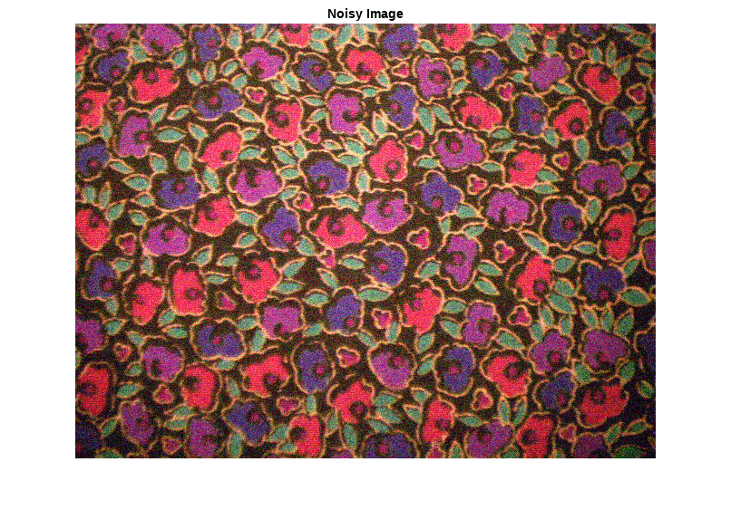
Use the imnoise (Image Processing Toolbox) function to add zero-mean Gaussian white noise with a variance of 0.00001 to the reference image.

Inoisy = imnoise(Ireference,"gaussian",0.00001);
imshow(Inoisy)
title("Noisy Image")

Filter Image Using Bilateral Filtering

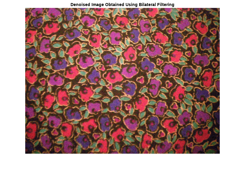
Conventional bilateral filtering is a standard way to reduce image noise while preserving edge sharpness. Use the imbilatfilt (Image Processing Toolbox) function to apply a bilateral filter to the noisy image. Specify a degree of smoothing equal to the variance of pixel values.

degreeOfSmoothing = var(double(Inoisy(:)));
Ibilat = imbilatfilt(Inoisy,degreeOfSmoothing);
imshow(Ibilat)
title("Denoised Image Obtained Using Bilateral Filtering")

Process Image Using Trained Network

Pass the normalized input image through the trained network and observe the output. The output of the network is the desired denoised image, returned as a dlarray object. Extract the image data from the dlarray object by using the extractdata function.

InoisyDL = dlarray(single(Inoisy),"SSCB");
IapproxDL = predict(net,InoisyDL);
Iapprox = extractdata(IapproxDL);

Image Processing Toolbox™ requires floating point images to have pixel values in the range [0, 1]. Use the rescale function to scale the pixel values to this range, then convert the image to uint8.

Iapprox = rescale(Iapprox);
Iapprox = im2uint8(Iapprox);
imshow(Iapprox)
title("Denoised Image Obtained Using Multiscale CAN")

Visual Comparison

To get a better visual understanding of the denoised images, examine a small region inside each image. Specify a region of interest (ROI) using vector roi in the format [x y width height]. The elements define the x- and y-coordinate of the top left corner, and the width and height of the ROI.

roi = [300 30 50 50];

Crop the images to this ROI, and display the result as a montage. The CAN removes more noise than conventional bilateral filtering. Both techniques preserve edge sharpness.

montage({imcrop(Ireference,roi),imcrop(Inoisy,roi), ...
    imcrop(Ibilat,roi),imcrop(Iapprox,roi)}, ...
    Size=[1 4]);
title("Reference Image | Noisy Image | Bilateral-Filtered Image | CAN Prediction");

Quantitative Comparison

Use image quality metrics to quantitatively compare the noisy input image, the bilateral-filtered image, and the operator-approximated image. The reference image is the original reference image, Ireference, before adding noise.

Measure the peak signal-to-noise ratio (PSNR) of each image against the reference image. Larger PSNR values generally indicate better image quality. See psnr (Image Processing Toolbox) for more information about this metric.

noisyPSNR = psnr(Inoisy,Ireference);
bilatPSNR = psnr(Ibilat,Ireference);
approxPSNR = psnr(Iapprox,Ireference);
PSNR_Score = [noisyPSNR bilatPSNR approxPSNR]';

Measure the structural similarity index (SSIM) of each image. SSIM assesses the visual impact of three characteristics of an image: luminance, contrast and structure, against a reference image. The closer the SSIM value is to 1, the better the test image agrees with the reference image. See ssim (Image Processing Toolbox) for more information about this metric.

noisySSIM = ssim(Inoisy,Ireference);
bilatSSIM = ssim(Ibilat,Ireference);
approxSSIM = ssim(Iapprox,Ireference);
SSIM_Score = [noisySSIM bilatSSIM approxSSIM]';

Measure perceptual image quality using the Naturalness Image Quality Evaluator (NIQE). Smaller NIQE scores indicate better perceptual quality. See niqe (Image Processing Toolbox) for more information about this metric.

noisyNIQE = niqe(Inoisy);
bilatNIQE = niqe(Ibilat);
approxNIQE = niqe(Iapprox);
NIQE_Score = [noisyNIQE bilatNIQE approxNIQE]';

Display the metrics in a table.

table(PSNR_Score,SSIM_Score,NIQE_Score, ...
    RowNames=["Noisy Image","Bilateral Filtering","Operator Approximation"])

ans=3×3 table
                              PSNR_Score    SSIM_Score    NIQE_Score
                              __________    __________    __________

    Noisy Image                 20.276       0.76228        11.574  
    Bilateral Filtering         25.753       0.91534         6.924  
    Operator Approximation      26.173       0.92976        5.8165

References

[1] Chen, Q. J. Xu, and V. Koltun. "Fast Image Processing with Fully-Convolutional Networks." In Proceedings of the 2017 IEEE Conference on Computer Vision. Venice, Italy, Oct. 2017, pp. 2516-2525.

[2] Grubinger, M., P. Clough, H. Müller, and T. Deselaers. "The IAPR TC-12 Benchmark: A New Evaluation Resource for Visual Information Systems." Proceedings of the OntoImage 2006 Language Resources For Content-Based Image Retrieval. Genoa, Italy. Vol. 5, May 2006, p. 10.