Generate RoadRunner Scene with Trees and Buildings Using Recorded Lidar Data
This example shows how to generate a High-Definition (HD) scene containing static objects, such as buildings, trees, cones, and other road side objects, by using labeled lidar data.
You can create a virtual scene from recorded sensor data that represents real-world scenes containing roadside objects and use it to perform verification of automated driving functionality, including sensor model validation. Lidar point clouds enable you to accurately extract the dimensions of the static objects surrounding the ego vehicle. Using this extracted information, you can create a high-definition scene in RoadRunner that contains objects such as trees and buildings.
In this example, you:
Load, explore, and visualize recorded driving data.
Register the point cloud.
Extract the location, dimension, and orientation information of the static objects.
Create a RoadRunner Scene.
Build and view the RoadRunner Scene.
Load Sensor Data
This example requires the Scenario Builder for Automated Driving Toolbox™ support package. Check if the support package is installed and, if it is not installed, install it using the Get and Manage Add-Ons.
checkIfScenarioBuilderIsInstalled
Download a ZIP file containing a subset of sensor data from the PandaSet data set, and then unzip the file. This file contains data for a continuous sequence of 80 point clouds and images. The images are for visual comparison only. The data also contains segmentation labels, consisting of an RGB triplet for each point in the point cloud, as well as the lidar sensor pose, and GPS data corresponding to each timestamp. The point clouds are labeled according to the color label triplets as defined in the helperLidarColorMap helper function.
dataFolder = tempdir;
lidarDataFileName = "PandasetStaticObjectsData.zip";
url = "https://ssd.mathworks.com/supportfiles/driving/data/" + lidarDataFileName;
filePath = fullfile(dataFolder,lidarDataFileName);
if ~isfile(filePath)
    websave(filePath,url);
end
unzip(filePath,dataFolder)
Create a datastore containing all PCD files within the specified folder by using the fileDatastore object, and read these files by using the pcread function. Sensor timestamps are in microseconds. Convert them to seconds, and offset the data from the first timestamp. Then, create a table containing the path to the lidar point cloud file, as well as the segmentation label, heading, and pose of the lidar sensor and GPS data corresponding to each timestamp.
lidarFilePath = fullfile(dataFolder,"Lidar");
pcds = fileDatastore(lidarFilePath,ReadFcn=@pcread);

% Load the images corresponding to each timestamp for visual comparison.
cameraFilePath = fullfile(dataFolder,"Camera");
imds = fileDatastore(cameraFilePath,ReadFcn=@imread);

% load the timestamps, segmentation labels, headings, and positions of the lidar sensor and GPS data.
load(fullfile(dataFolder,"sensorData.mat"))

% The timestamps of the sensor are in microseconds. Convert to seconds and offset from the first timestamp.
tsecs = timestamps*(1e-6);
tsecs = tsecs - tsecs(1);

% Create a table containing the path to the lidar point cloud file, as well as the
% segmentation label, heading, and pose of the lidar sensor and GPS data corresponding to each timestamp.
varNames = ["Timestamps","CameraPath","LidarPath","Labels","Heading","Position","GPS"];
lidarData = table(tsecs,imds.Files,pcds.Files,labels,heading,position,gps,VariableNames=varNames);
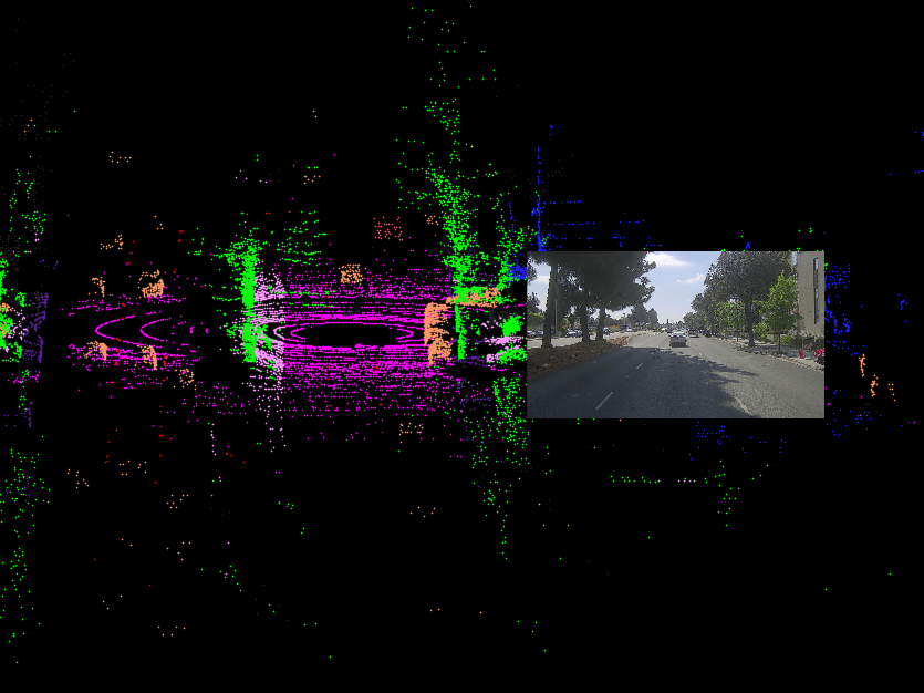
Read and display the first point cloud and corresponding labels from the lidarData table. Remove the points with Inf or NaN coordinate values from the point cloud using removeInvalidPoints. An integer represents the segmentation label for each point in the point cloud in the data. The helperLidarColorMap defines the corresponding RGB triplet for each integer label.
% Read the point cloud corresponding to the first timestamp.
ptCld = pcread(lidarData.LidarPath{1});
% Remove points with Inf or NaN coordinate values from the point cloud.
[ptCld,indices] = removeInvalidPoints(ptCld);

% Read the segmentation labels corresponding to the first timestamp, and select the labels corresponding to the valid points in the point cloud.
segLabels = lidarData.Labels{1};
labelsUnorg = segLabels(indices);

% Use helperLidarColorMap to color the point cloud based on the segmentation labels.
cmap = helperLidarColorMap;
color = cell2mat(cmap(labelsUnorg));
ptCld.Color = uint8(color);

% Read the image corresponding to the first timestamp for visual comparison.
img = imread(lidarData.CameraPath{1});

% Visualize the lidar and camera data of the first frame.
helperVisualizePointCloud(ptCld,img)
Register Point Clouds
In this example, the lidar point clouds for each frame are in sensor frame. Create a rigidtform3d using the rotation matrix and translation vector obtained from heading and position of the lidar sensor. Use the geometric transformation to transform the lidar point cloud from the sensor frame to the world frame. If the heading and position information of the lidar sensor is not available, you can register the point cloud data by using the iterative closest point (ICP) algorithm. For more information, see the 3-D Point Cloud Registration and Stitching example.
For each timestamp use the segmentation labels to select the points belonging to buildings, vegetation, and other roadside objects and store them in separate arrays.
% Store the labels of vegetation, pylons, buildings, and cones in an array. This corresponds to the colormap obtained from helperLidarColorMap.
labelIndices = [2 12 15 17];
Now, create empty point cloud arrays to store the point clouds for the different types of objects, and extract the points into their respective arrays, based on their segmentation labels. Finally, concatenate the point cloud array for each object type to create a single point cloud for that object type for the entire scene, and store all the point clouds in a cell array.
sz = size(lidarData);
pcVegetation = pointCloud.empty(sz(1),0);
pcPylons = pointCloud.empty(sz(1),0);
pcBuildings = pointCloud.empty(sz(1),0);
pcCones = pointCloud.empty(sz(1),0);

pointClouds = {pcVegetation;
    pcPylons;
    pcBuildings;
    pcCones};

% Color the point cloud based on the segmentation labels using the helperLidarColorMap function.
cmap = helperLidarColorMap;

for i = 1:size(lidarData,1)
    % Read the current frame.
    ptCld = pcread(lidarData.LidarPath{i});
    % Remove points with Inf or NaN coordinate values from the point cloud.
    [ptCld,indices] = removeInvalidPoints(ptCld);

    % Use ground truth labels to color each point in the point cloud.
    segLabels = lidarData.Labels{i};
    labelsUnorg = segLabels(indices);
    color = cell2mat(cmap(labelsUnorg));
    ptCld.Color = uint8(color);

    % Create a 3D rigid geometric transformation using lidar pose.
    rot = rotmat(quaternion(lidarData.Heading(i,:)),"point");
    tran = lidarData.Position(i,:);
    tform = invert(rigidtform3d(rot,tran));

    % Transform the point cloud to world coordinates using the geometric transformation.
    ptCldOut = pctransform(ptCld,tform);

    % Select the point clouds belonging to each static object and store
    % them in the corresponding cell of the cell array.
    for j = 1:length(labelIndices)
        % Get the indices of the point clouds for each type of static object by using the Color property.
        idx = all(ptCldOut.Color == cell2mat(cmap(labelIndices(j))),2);

        % Store the point clouds in the cell array.
        pointClouds{j} = [pointClouds{j}; select(ptCldOut,idx)];
    end
end

% Concatenate each point cloud array to create a single point cloud for
% each corresponding static object.
for j = 1:length(pointClouds)
    pointClouds{j} = pccat(pointClouds{j});
end
Extract Trees and Buildings from Registered Point Cloud
To generate a RoadRunner Scene, you must have a cuboid parameters array for each instance of the static object.
For each type of static object, obtain clusters of point clouds using the pcsegdist function. Use the minDistance argument to set the minimum distance between points of two different clusters, and the NumClusterPoints argument to set the minimum number of points to include in each cluster based on the density of points in the registered point cloud of each static object. Then, fit a cuboid model to each cluster using the pcfitcuboid (Lidar Toolbox) function, and store the location and dimension parameters of each cluster in an array. Store the parameters of the cuboid models for each type of static object.
% Initialize parameters to segment point clouds into clusters based on Euclidean distance.
% The order of labels is same as that of labelIndices.
minDistanceArray = [0.5 0.3 0.3 0.5];     % Minimum Euclidean distance between points from two clusters.
NumClusterPointsArray = [300 50 500 10];  % Minimum number of points in each cluster.

% Create an empty cell array to store the parameters of the cuboids.
cuboids = cell(size(labelIndices,2),1);

for i = 1:length(pointClouds)
    ptCloud = pointClouds{i};
    minDistance = minDistanceArray(i);
    NumClusterPoints = NumClusterPointsArray(i);

    [labels,numClusters] = pcsegdist(ptCloud,minDistance,NumClusterPoints=NumClusterPoints);

    for j = 1:numClusters
        % Find the indices of points within the same cluster.
        idx = find(j == labels);

        % Fit the cuboid model to each cluster.
        model = pcfitcuboid(ptCloud,idx);

        % Store the model in the array.
        cuboids{i} = [cuboids{i}; model.Parameters];
    end
end
Visualize the cuboids of the static objects by overlaying them on the point clouds.
titleArray = {"Vegetation Cuboids","Pylons Cuboids","Buildings Cuboids","Cones Cuboids"};
f = figure(Position=[1182 696 1000 800]);
for i = 1:length(pointClouds)
    ptCloud = pointClouds{i};
    cuboidParameters = cuboids{i};
    ax = subplot(2,2,i);
    pcshow(pointClouds{i},Parent=ax)
    showShape(cuboid=cuboids{i},Parent=ax,color="red",Opacity=0.1)
    view(0,90)
    title(ax,titleArray{i})
end
Create RoadRunner HD Map
Create an empty RoadRunner HD Map.
rrMap = roadrunnerHDMap;
For better visualization of the generated scene, add road data to the map before adding static objects. For more information on creating road data, see the Generate RoadRunner Scene Using Labeled Camera Images and Raw Lidar Data example.
filename = fullfile(dataFolder,"mapWithRoad.rrhd");
read(rrMap,filename)
Set the geographic reference of the HD Map to the start of the sequence. If GPS data is not available, instead set the geographic reference to [0 0].
rrMap.GeoReference = [lidarData.GPS(1,1),lidarData.GPS(1,2)];
Store the cuboid parameters for the different types of static objects in a structure.
staticObjects.trees = cuboids{1};
staticObjects.pylons = cuboids{2};
staticObjects.buildings = cuboids{3};
staticObjects.cones = cuboids{4};
Generate static object information in the RoadRunner HD Map format by using the roadrunnerStaticObjectInfo function.
objectsInfo = roadrunnerStaticObjectInfo(staticObjects);
Update the map with information of the static object information.
rrMap.StaticObjectTypes = objectsInfo.staticObjectTypes;
rrMap.StaticObjects = objectsInfo.staticObjects;
Plot the map, which contains information for the static objects, lane boundaries, and lane centers.
f = figure(Position=[1000 818 700 500]);
ax = axes("Parent",f);
plot(rrMap,ShowStaticObjects=true,Parent=ax)
Write the RoadRunner HD Map to a binary file, which you can import into the Scene Builder Tool.
write(rrMap,"RoadSideObjectsScene.rrhd")Build RoadRunner Scene
Open the RoadRunner application by using the roadrunner (RoadRunner) object. Import the RoadRunner HD Map data from your binary file, and build it in the currently open scene.
Specify the path to your local RoadRunner installation folder. This code shows the path for the default installation location on Windows®.
rrAppPath = "C:\Program Files\RoadRunner " + "R2025a" + "\bin\win64";
Specify the path to your RoadRunner project. This code shows the path to a sample project folder on Windows.
rrProjectPath = "C:\RR\MyProject";Open RoadRunner using the specified path to your project
rrApp = roadrunner(rrProjectPath,InstallationFolder=rrAppPath);
Copy the RoadRunnerHDMap.rrhd scene file into the asset folder of RoadRunner project and import it into RoadRunner.
copyfile("RoadSideObjectsScene.rrhd",(rrProjectPath + filesep + "Assets"))
file = fullfile(rrProjectPath,"Assets","RoadSideObjectsScene.rrhd");
importScene(rrApp,file,"RoadRunner HD Map")
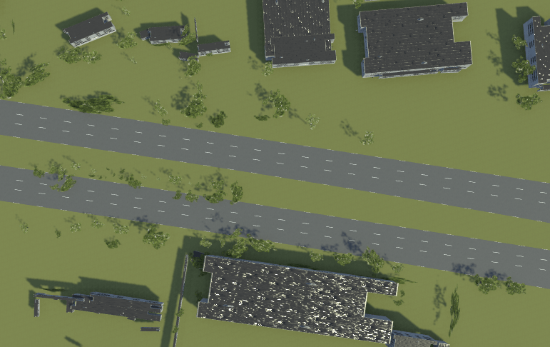
This figure shows a scene built using the Scene Builder Tool.
Note: Use of the Scene Builder Tool requires a RoadRunner Scene Builder license, and use of RoadRunner Assets requires a RoadRunner Asset Library Add-On license.

To visually compare the generated scene with the actual scene, use the satellite view of the geographic player.
% Set the center of the geographic player at the center frame of the sequence.
sequenceCenter = size(lidarData,1)/2;
latCenter = lidarData.GPS(sequenceCenter,1);
lonCenter = lidarData.GPS(sequenceCenter,2);
zoomLevel = 18;
player = geoplayer(latCenter,lonCenter,zoomLevel,Basemap="satellite");
Helper Functions
helperLidarColorMap — Color map for the lidar labels.
function cmap = helperLidarColorMap
% This function contains the color map for all the lidar labels.
labels = [1:17]';

labelColors = {
    [30     30       30];   % UnClassified
    [0      255       0];   % Vegetation
    [255    150     255];   % Ground
    [255    0       255];   % Road
    [255    0         0];   % Road Markings
    [90     30      150];   % Side Walk
    [245    150     100];   % Car
    [250    80      100];   % Truck
    [150    60       30];   % Other Vehicle
    [255    255       0];   % Pedestrian
    [0      150     255];   % Animals
    [75     0        75];   % Pylons
    [0      200     255];   % Barricade
    [170    100     150];   % Signs
    [30     30      255];   % Building
    [60     60      100];   % ThrashBox
    [70     70      200]    % Cones
    };

    cmap = dictionary(labels, labelColors);

end
helperVisualizePointCloud — A helper function to plot the point cloud with camera view.
function helperVisualizePointCloud(ptCld,img)
figureFirstPointCloud = figure(Position=[350 180 800 600]);
subplot1 = subplot(1,2,1,Parent=figureFirstPointCloud);
hold on
pcshow(ptCld)
% Set axes properties for better visualization
set(subplot1,CameraPosition=[698 548 123], ...
    CameraTarget=[31.76 17.78 3.3], ...
    CameraViewAngle=1.51, ...
    Color=[0 0 0], ...
    PlotBoxAspectRatio=[12.12 13.26 1], ...
    Projection="perspective")
hold off
subplot2 = subplot(1,2,2,Parent=figureFirstPointCloud);
hold on
imshow(img)
hold off
end
References
[1] Hesai and Scale. PandaSet. Accessed September 18, 2025. https://pandaset.org/. The PandaSet data set is provided under the CC-BY-4.0 license.
See Also
Functions
roadrunnerLaneInfo|roadrunnerStaticObjectInfo|getMapROI|roadprops|selectActorRoads|updateLaneSpec|actorprops
Objects
Topics
- Overview of Scenario Generation from Recorded Sensor Data
- Generate RoadRunner Scene Using Processed Camera Data and GPS Data
- Generate RoadRunner Scene Using Labeled Camera Images and Raw Lidar Data
- Generate RoadRunner Scene from Recorded Lidar Data
- Generate RoadRunner Scenario from Recorded Sensor Data
- Extract Lane Information from Recorded Camera Data for Scene Generation
- Extract Vehicle Track List from Recorded Camera Data for Scenario Generation