procest

Estimate process model using time-domain or frequency-domain data

collapse all in page

Syntax

sys = procest(tt,type)

sys = procest(data,type)

sys = procest(___,Name,Value)

sys = procest(tt,init_sys)

sys = procest(data,init_sys)

sys = procest(___,opt)

[sys,offset] = procest(___)

[sys,offset,ic] = procest(___)

Description

Estimate Process Model

sys = procest(tt,type) estimates the process model sys using all the input and output signals in the timetable tt. type defines the structure of sys. You can use this syntax for SISO and MISO systems. The function assumes that the last variable in the timetable is the single output signal.

A simple SISO process model has a gain, a time constant, and a delay:

$s y s = \frac{K_{p}}{1 + T_{p 1} s} e^{- T_{d} s} .$

K_p is a proportional gain. T_p₁ is the time constant of the real pole, and T_d is the transport delay (dead time). More complex process models can include zeroes, additional time constants, complex poles, and integration. For more information on process models, see idproc.

You cannot use procest to estimate time-series models, which are models that contain no inputs. Use ar, arx, or armax for time-series models instead.

You cannot reliably estimate accurate process models from matrix-based data as you can with other model types. Process models are always continuous, and, because numeric matrices contain no sample time information, estimating continuous models from matrix-based data is generally not recommended. For information on converting matrices to timetables, see Convert SISO Matrix Data to Timetable.

example

sys = procest(data,type) uses the time-domain or frequency-domain data in data. Use this syntax especially when you want to estimate a process model using frequency-domain or frequency response data, or when you want to take advantage of the additional information, such as intersample behavior, data sample time, or experiment labeling, that data objects provide.

sys = procest(___,Name,Value) incorporates additional options specified by one or more name-value arguments. For example, sys = procest(tt,P1D,'InputDelay',2) specifies an input delay of 2. You can use this syntax with any of the previous input-argument combinations

example

Configure Initial Parameters

sys = procest(tt,init_sys) uses the process model init_sys to configure the initial parameterization for estimation using the timetable tt.

example

sys = procest(data,init_sys) uses the uses the data object data for estimation.

example

Specify Additional Options

sys = procest(___,opt) specifies additional model estimation options. Use opt with any of the input argument combinations in the previous syntaxes.

example

Return Estimated Offset and Initial Conditions

[sys,offset] = procest(___) returns the estimated value of the offset in input signal. procest automatically estimates the input offset when the model contains an integrator or when you set the InputOffset estimation option to 'estimate' using procestOptions.

example

[sys,offset,ic] = procest(___) returns the estimated initial conditions as an initialCondition object. Use this syntax if you plan to simulate or predict the model response using the same estimation input data and then compare the response with the same estimation output data. Incorporating the initial conditions yields a better match during the first part of the simulation.

example

Examples

collapse all

Estimate and Refine Process Model

Open Live Script

Estimate a process model and compare its response with the measured output.

Load the input/output data, which is stored in the timetable tt1.

load sdata1 tt1

Estimate a first-order process model sys that contains one pole and no zeroes or delays. This model structure has type P1.

sys = procest(tt1,'P1');

Compare the simulated model response with the measured output.

compare(tt1,sys)

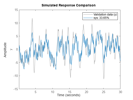
Figure contains an axes object. The axes object with ylabel y contains 2 objects of type line. These objects represent Validation data (y), sys: 33.65%.

The fit percentage for the model is low. Add a delay to the model and compare the simulated and measured outputs.

sys = procest(tt1,'P1D');
compare(tt1,sys)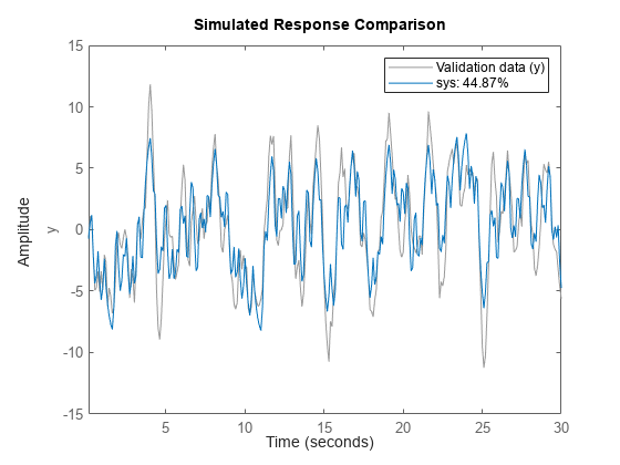

Figure contains an axes object. The axes object with ylabel y contains 2 objects of type line. These objects represent Validation data (y), sys: 44.87%.

The fit percentage has improved, but is still below 50%. The plot shows that the model output peaks do not attain the height of the measured output peaks, which indicates that the model needs to include more dynamics.

Create a second-order process model with complex (underdamped) poles.

sys = procest(tt1,'P2U');
compare(tt1,sys)

Figure contains an axes object. The axes object with ylabel y contains 2 objects of type line. These objects represent Validation data (y), sys: 70.44%.

The fit now exceeds 70%.

You can view more information about the estimation by exploring the idproc property sys.Report.

sys.Report

ans = 
              Status: 'Estimated using PROCEST'
              Method: 'PROCEST'
    InitialCondition: 'zero'
                 Fit: [1x1 struct]
          Parameters: [1x1 struct]
         OptionsUsed: [1x1 idoptions.procest]
           RandState: []
            DataUsed: [1x1 struct]
         Termination: [1x1 struct]

View the estimated gain Kp.

Kp = sys.Kp

Kp = 
7.6818

Specify Parameter Initial Values for Estimated Process Model

Open Live Script

Estimate a process model after specifying initial guesses for parameter values and bounding them.

Obtain input/output data.

data = idfrd(idtf([10 2],[1 1.3 1.2],'iod',0.45),logspace(-2,2,256));

Specify the parameters of the estimation initialization model.

type = 'P2UZD';
init_sys = idproc(type);

init_sys.Structure.Kp.Value = 1; 
init_sys.Structure.Tw.Value = 2; 
init_sys.Structure.Zeta.Value = 0.1; 
init_sys.Structure.Td.Value = 0; 
init_sys.Structure.Tz.Value = 1; 
init_sys.Structure.Kp.Minimum = 0.1;
init_sys.Structure.Kp.Maximum = 10;
init_sys.Structure.Td.Maximum = 1;
init_sys.Structure.Tz.Maximum = 10;

Specify the estimation options.

opt = procestOptions('Display','full','InitialCondition','Zero');
opt.SearchMethod = 'lm'; 
opt.SearchOptions.MaxIterations = 100;

Estimate the process model.

sys = procest(data,init_sys,opt);

Since the 'Display' option is specified as 'full', the estimation progress is displayed in a separate Plant Identification Progress window.

Compare the data to the estimated model.

compare(data,sys);

Figure contains 2 axes objects. Axes object 1 with title From: u1, ylabel To: y1 contains 2 objects of type line. These objects represent Data, sys: 100%. Axes object 2 with ylabel To: y1 contains 2 objects of type line. These objects represent Data, sys: 100%.

Return Input Offsets Estimated During Process Model Estimation

Open Live Script

load iddata1
[sys,offset] = procest(z1,'P1DI');
offset

offset = 
0.0412

Obtain Initial Conditions

Open Live Script

Load the data.

load iddata1ic z1i

Estimate a first-order plus dead time process model sys and return the initial conditions in ic. First specify 'estimate' for 'InitialCondition' to force the software to estimate ic. The default 'auto' setting uses the 'estimate' method only when the influence of the initial conditions on the overall model error exceed a threshold. When the initial conditions have a negligible effect on the overall estimation-error minimization process, the 'auto' setting uses 'zero'.

opt = procestOptions('InitialCondition','estimate');
[sys,offset,ic] = procest(z1i,'P1D',opt);
ic

ic = 
  initialCondition with properties:

     A: -3.8997
    X0: -1.0871
     C: 4.5652
    Ts: 0

ic is an initialCondition object that encapsulates the free response of sys, in state-space form, to the initial state vector in X0. You can incorporate ic when you simulate sys with the z1i input signal and compare the response with the z1i output signal.

Detect Overparameterization of Estimated Model

Open Live Script

Obtain input/output data.

load iddata1 z1
load iddata2 z2
data = [z1 z2(1:300)];

data is a data set with 2 inputs and 2 outputs. The first input affects only the first output. Similarly, the second input affects only the second output.

In the estimated process model, the cross terms, which model the effect of the first input on the second output and vice versa, should be negligible. If the estimation process instead assigns higher orders to the cross dynamics, the degrees of estimation uncertainty for those terms should be high.

Estimate the process model.

type = 'P2UZ'; 
sys = procest(data,type);

The type variable denotes a model with complex-conjugate pair of poles, a zero, and a delay.

To evaluate the uncertainties, plot the frequency response.

w = linspace(0,20*pi,100);
h = bodeplot(sys,w);
showConfidence(h);

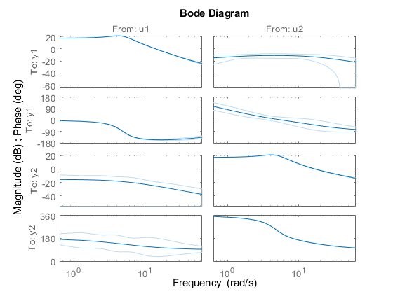
The responses from the cross pairs show larger uncertainty, indicating that using a single type for each input/output pair results in too much energy in the cross pairs.

Estimate Overparameterized Process Model Using Regularization

Open Live Script

Use regularization to estimate parameters of an overparameterized process model.

Load the data.

load iddata1 z1;

Construct an initial system sysi by specifying parameter values for a model that includes three poles, one zero, and underdamped modes. Assume that gain Kp is known with a higher degree of confidence than the other model parameters.

sysi = idproc('P3UZ','Kp',7.5,'Tw',0.25,'Zeta',0.3,'Tp3',20,'Tz',0.02);

Estimate an unregularized process model sys1 using sysi to initialize the estimation model.

sys1 = procest(z1,sysi);

Estimate a regularized process model sys2 from sysi. Because K has a higher level of confidence, set the regularization constant R higher than for the other model parameters. This setting causes the estimation process to place more emphasis on maintaining the initial value of K.

opt = procestOptions;
opt.Regularization.Nominal = 'model';
opt.Regularization.R = [100;1;1;1;1];
opt.Regularization.Lambda = 0.1;
sys2 = procest(z1,sysi,opt);

Compare the model outputs with data.

compare(z1,sys1,sys2);

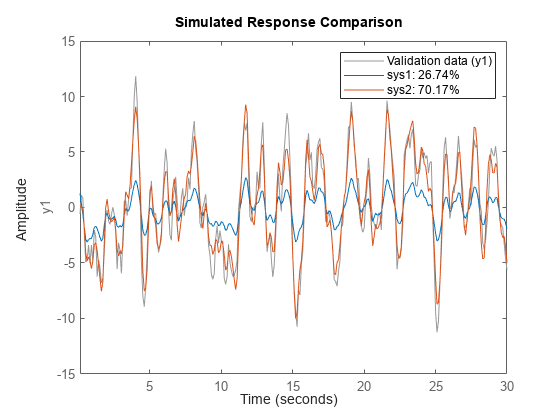
Figure contains an axes object. The axes object with ylabel y1 contains 3 objects of type line. These objects represent Validation data (y1), sys1: 26.74%, sys2: 70.16%.

Regularization helps steer the estimation process towards the correct parameter values, as the better fit for sys2 shows.

Compare the estimated gain values for sys1 and sys2.

g1 = sys1.Kp

g1 = 
-0.2320

g2 = sys2.Kp

g2 = 
6.6236

The Kp value for the regularized system is much closer to the initial value than for the unregularized system.

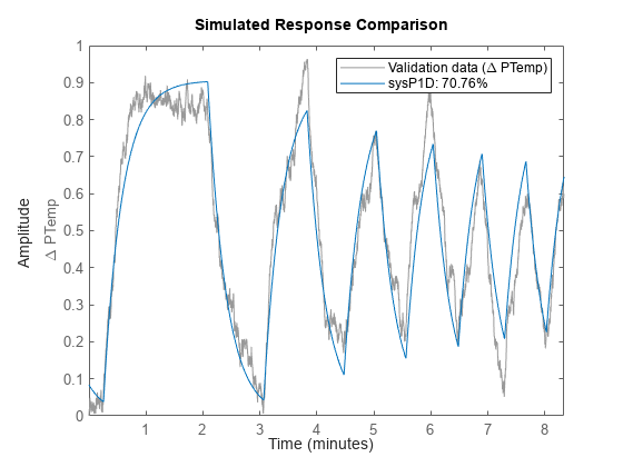
Estimate a First Order Plus Dead Time Model

Open Live Script

Obtain the measured input-output data.

load iddemo_heatexchanger_data;
data = iddata(pt,ct,Ts);  
data.InputName  = '\Delta CTemp';
data.InputUnit  = 'C';
data.OutputName = '\Delta PTemp';
data.OutputUnit = 'C';
data.TimeUnit   = 'minutes';

Estimate a first-order plus dead time process model.

type = 'P1D';
sysP1D = procest(data,type);

Compare the model with the data.

compare(data,sysP1D)

$Figure contains an axes object. The axes object with ylabel Delta PTemp contains 2 objects of type line. These objects represent Validation data (\Delta PTemp), sysP1D: 70.76%.$

Plot the model residuals.

figure
resid(data,sysP1D);

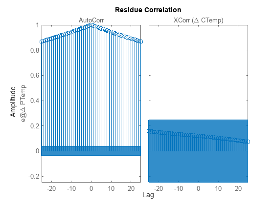
$Figure contains 2 axes objects. Axes object 1 with title AutoCorr, ylabel e@\Delta PTemp contains 2 objects of type line. One or more of the lines displays its values using only markers This object represents sysP1D. Axes object 2 with title XCorr ( Delta blank CTemp) contains 2 objects of type line. One or more of the lines displays its values using only markers This object represents sysP1D.$

The figure shows that the residuals are correlated. To account for that, add a first order ARMA disturbance component to the process model.

opt = procestOptions('DisturbanceModel','ARMA1');
sysP1D_noise = procest(data,'p1d',opt);

Compare the models.

compare(data,sysP1D,sysP1D_noise)

$Figure contains an axes object. The axes object with ylabel Delta PTemp contains 3 objects of type line. These objects represent Validation data (\Delta PTemp), sysP1D: 70.76%, sysP1D\_noise: 24.43%.$

Plot the model residuals.

figure
resid(data,sysP1D_noise);

$Figure contains 2 axes objects. Axes object 1 with title AutoCorr, ylabel e@\Delta PTemp contains 2 objects of type line. One or more of the lines displays its values using only markers This object represents sysP1D\_noise. Axes object 2 with title XCorr ( Delta blank CTemp) contains 2 objects of type line. One or more of the lines displays its values using only markers This object represents sysP1D\_noise.$

The residues of sysP1D_noise are uncorrelated.

Input Arguments

collapse all

`tt` — Timetable-based estimation data
`timetable` | cell array of `timetables`

Estimation data, specified as a uniformly sampled timetable that contains both input and output signal variables or, for multiexperiment data, a cell array of timetables.

Use Entire Timetable

If you want to use all the input and output variables in tt, and the variables are organized so that the set of input variables is followed by the set of output variables, then:

For SISO systems, specify tt as an N_s-by-2 timetable, where N_s is the number of samples and the two timetable variables represent the measured input signal and output signal respectively.
For MIMO systems, specify tt as an N_s-by-(N_u+N_y) timetable, where N_u is the number of inputs and N_y is the number of outputs. The first N_u variables must contain the input signals and the remaining N_y variables must contain the output signals.
When you are estimating state space or transfer function models, you must also explicitly specify the input and output channels, as the following section describes.
For multiexperiment data, specify data as an N_e-by-1 cell array of timetables, where N_e is the number of experiments. The sample times of all the experiments must match.

Use Selected Variables from Timetable

If you want to use a subset of variables from the timetable, or if the input and output variables are intermixed, use the 'InputName' and 'OutputName' name-value arguments to specify which variables to use.

For example, suppose that tt contains six variables: "u1", "u2", "u3", and "y1", "y2", "y3". For estimation, you want to use the variables "u1" and "u2" as the inputs and the variables "y1" and "y3" as the outputs. Use the following command to perform the estimation:

sys = procest(tt,__,'InputName',["u1" "u2"],'OutputName',["y1" "y3"])

For more information about working with estimation data types, see Data Domains and Data Types in System Identification Toolbox.

`data` — Estimation data object
`iddata` object | `frd` object | `idfrd` object

Estimation data object, specified as an iddata object, an frd object, or an idfrd object that contains uniformly sampled input and output values. By default, the software sets the sample time of the model to the sample time of the estimation data.

For multiexperiment data, the sample times and intersample behavior of all the experiments must match.

For time-domain estimation, data must be an iddata object containing the input and output signal values.

For frequency-domain estimation, data can be one of the following:

Recorded frequency response data (frd (Control System Toolbox) or idfrd)
iddata object with properties specified as follows:
- InputData — Fourier transform of the input signal
- OutputData — Fourier transform of the output signal
- Domain — 'Frequency'

Limitations

You cannot estimate continuous-time models using discrete-time frequency-domain data.

`type` — Process model structure
character vector | string | cell array of character vectors | string array

Process model structure, specified for SISO models as a string or character vector that represents an acronym for the model structure, such as 'P1D' or 'P2DZ'. The acronym starts with P and can contain any combination of the other following components:

P — Poles. All 'Type' acronyms start with P, because all process modes must have at least one pole.
0, 1, 2, or 3 — Number of time constants (poles) to be modeled. This number does not include possible integrations (poles in the origin).
I — Integration is enforced (self-regulating process).
D — Time delay (dead time).
Z — Extra numerator term, a zero.
U — Underdamped modes (complex-valued poles) permitted. If U is not included in type, all poles must be real. The number of poles must be 2 or 3.

For MIMO models, specify type as an Ny-by-Nu cell array of character vectors or string array, with one entry for each input-output pair. Here Ny is the number of inputs and Nu is the number of outputs.

For information regarding how type affects the structure of a process model, see idproc.

`init_sys` — Process model that configures initial parameterization of `sys`
`idproc` object

Process model that configures initial parameterization of sys, specified as an idproc object. You obtain init_sys by either performing an estimation using measured data or by direct construction using idproc. The software uses the parameters and constraints defined in init_sys as the initial guess for estimating sys.

Use the Structure property of init_sys to configure initial guesses and constraints for K_p, T_p1, T_p2, T_p3, T_w, ζ, T_d, and T_z. For example:

To specify an initial guess for the T_p1 parameter of init_sys, set init_sys.Structure.Tp1.Value as the initial guess.
To specify constraints for the T_p2 parameter of init_sys:
- Set init_sys.Structure.Tp2.Minimum to the minimum T_p2 value.
- Set init_sys.Structure.Tp2.Maximum to the maximum T_p2 value.
- Set init_sys.Structure.Tp2.Free to indicate if T_p2 is a free parameter for estimation.

If you do not specify opt, and init_sys was obtained by estimation rather than construction, then the software uses estimation options from init_sys.Report.OptionsUsed

`opt` — Estimation options
`procestOptions` option set

Estimation options, specified as an procestOptions option set. The estimation options include:

Estimation objective
Handling on initial conditions and disturbance component
Numerical search method to be used in estimation
Intersample behavior

Name-Value Arguments

Specify optional pairs of arguments as Name1=Value1,...,NameN=ValueN, where Name is the argument name and Value is the corresponding value. Name-value arguments must appear after other arguments, but the order of the pairs does not matter.

Before R2021a, use commas to separate each name and value, and enclose Name in quotes.

Example: sys = procest(tt,'P1D,'InputDelay',2)

`InputName` — Input channel names
string | character vector | string array | cell array of character vectors

Input channel names, specified as a string, character vector, string array, or cell array of character vectors.

If you are using a timetable for the data source, the names in InputName must be a subset of the timetable variables.

Example: sys = procest(tt,__,'InputName',["u1" "u2"]) selects the variables u1 and u2 as the input channels from the timetable tt to use for the estimation.

`OutputName` — Output channel names
string | character vector | string array | cell array of character vectors

Output channel names, specified as a string, character vector, string array, or cell array of character vectors.

If you are using a timetable for the data source, the names in OutputName must be a subset of the timetable variables.

Example: sys = procest(tt,__,'OutputName',["y1" "y3"]) selects the variables y1 and y3 as the output channels from the timetable tt to use for the estimation.

`InputDelay` — Input delays
`0` for all input channels (default) | numeric vector

Input delays, specified as a numeric vector specifying a time delay for each input channel. Specify input delays in the time unit stored in the TimeUnit property.

For a system with Nu inputs, set InputDelay to an Nu-by-1 vector. Each entry of this vector is a numerical value that represents the input delay for the corresponding input channel. You can also set InputDelay to a scalar value to apply the same delay to all channels.

The software treats InputDelay as a fixed delay that is separate from any transport delay that the Td property of the model introduces.

Output Arguments

collapse all

`sys` — Identified process model
`idproc` model

Identified process model, returned as an idproc model of a structure defined by type.

Information about the estimation results and options used is stored in the model's Report property. Report has the following fields:

Report Field Description

Status

Summary of the model status, which indicates whether the model was created by construction or obtained by estimation

Method

Estimation command used

InitialCondition

Handling of initial conditions during model estimation, returned as one of the following values:

'zero' — The initial conditions were set to zero.
'estimate' — The initial conditions were treated as independent estimation parameters.
'backcast' — The initial conditions were estimated using the best least squares fit.

This field is especially useful to view how the initial conditions were handled when the InitialCondition option in the estimation option set is 'auto'.

Fit

Quantitative assessment of the estimation, returned as a structure. See Loss Function and Model Quality Metrics for more information on these quality metrics. The structure has these fields.

FitPercent — Normalized root mean squared error (NRMSE) measure of how well the response of the model fits the estimation data, expressed as the percentage fitpercent = 100(1-NRMSE)
LossFcn — Value of the loss function when the estimation completes
MSE — Mean squared error (MSE) measure of how well the response of the model fits the estimation data
FPE — Final prediction error for the model
AIC — Raw Akaike Information Criteria (AIC) measure of model quality
AICc — Small-sample-size corrected AIC
nAIC — Normalized AIC
BIC — Bayesian Information Criteria (BIC)

Parameters

Estimated values of model parameters

OptionsUsed

Option set used for estimation. If no custom options were configured, this is a set of default options. See procestOptions for more information.

RandState

State of the random number stream at the start of estimation. Empty, [], if randomization was not used during estimation. For more information, see rng.

DataUsed

Attributes of the data used for estimation. Structure with the following fields:

Field	Description
`Name`	Name of the data set.
`Type`	Data type. For `idnlarx` models, this is set to `'Time domain data'`.
`Length`	Number of data samples.
`Ts`	Sample time. This is equivalent to `Data.Ts`.
`InterSample`	Input intersample behavior. One of the following values: `'zoh'` — Zero-order hold maintains a piecewise-constant input signal between samples. `'foh'` — First-order hold maintains a piecewise-linear input signal between samples. `'bl'` — Band-limited behavior specifies that the continuous-time input signal has zero power above the Nyquist frequency. The value of `Intersample` has no effect on estimation results for discrete-time models.
`InputOffset`	Empty, `[]`, for nonlinear estimation methods.
`OutputOffset`	Empty, `[]`, for nonlinear estimation methods.

Termination

Termination conditions for the iterative search used for prediction error minimization, returned as a structure with these fields.

WhyStop — Reason for terminating the numerical search
Iterations — Number of search iterations performed by the estimation algorithm
FirstOrderOptimality — $\infty$ -norm of the gradient search vector when the search algorithm terminates
FcnCount — Number of times the objective function was called
UpdateNorm — Norm of the gradient search vector in the last iteration. Omitted when the search method is 'lsqnonlin' or 'fmincon'.
LastImprovement — Criterion improvement in the last iteration, expressed as a percentage. Omitted when the search method is 'lsqnonlin' or 'fmincon'.
Algorithm — Algorithm used by 'lsqnonlin' or 'fmincon' search method. Omitted when other search methods are used.

For estimation methods that do not require numerical search optimization, the Termination field is omitted.

For more information on using Report, see Estimation Report.

`offset` — Estimated value of input offset
vector

Estimated value of input offset, returned as a vector. When data has multiple experiments, offset is a matrix where each column corresponds to an experiment.

`ic` — Initial conditions
`initialCondition` object | object array of `initialCondition` values

Estimated initial conditions, returned as an initialCondition object or an object array of initialCondition values.

For a single-experiment data set, ic represents, in state-space form, the free response of the process model (A and C matrices) to the estimated initial states (x₀).
For a multiple-experiment data set with N_e experiments, ic is an object array of length N_e that contains one set of initialCondition values for each experiment.

If procest returns ic values of 0 and the you know that you have non-zero initial conditions, set the 'InitialCondition' option in procestOptions to 'estimate' and pass the updated option set to procest. For example:

opt = procestOptions('InitialCondition','estimate')
[sys,offset,ic] = procest(data,type,opt)

The default 'auto' setting of 'InitialCondition' uses the 'zero' method when the initial conditions have a negligible effect on the overall estimation-error minimization process. Specifying 'estimate' ensures that the software estimates values for ic.

For more information, see initialCondition. For an example of using this argument, see Obtain Initial Conditions.

Version History

Introduced in R2012a

expand all

R2022b: Time-domain estimation data is accepted in the form of timetables and matrices

Most estimation, validation, analysis, and utility functions now accept time-domain input/output data in the form of a single timetable that contains both input and output data or a pair of matrices that contain the input and output data separately. These functions continue to accept iddata objects as a data source as well, for both time-domain and frequency-domain data.

R2018a: Advanced Options are deprecated for `SearchOptions` when `SearchMethod` is `'lsqnonlin'`

Specification of lsqnonlin- related advanced options are deprecated, including the option to invoke parallel processing when estimating using the lsqnonlin search method, or solver, in Optimization Toolbox™.

procest

Syntax

Description

Estimate Process Model

Configure Initial Parameters

Specify Additional Options

Return Estimated Offset and Initial Conditions

Examples

Estimate and Refine Process Model

Specify Parameter Initial Values for Estimated Process Model

Return Input Offsets Estimated During Process Model Estimation

Obtain Initial Conditions

Detect Overparameterization of Estimated Model

Estimate Overparameterized Process Model Using Regularization

Estimate a First Order Plus Dead Time Model

Input Arguments

`tt` — Timetable-based estimation data
`timetable` | cell array of `timetables`

Use Entire Timetable

Use Selected Variables from Timetable

`data` — Estimation data object
`iddata` object | `frd` object | `idfrd` object

Limitations

`type` — Process model structure
character vector | string | cell array of character vectors | string array

`init_sys` — Process model that configures initial parameterization of `sys`
`idproc` object

`opt` — Estimation options
`procestOptions` option set

Name-Value Arguments

`InputName` — Input channel names
string | character vector | string array | cell array of character vectors

`OutputName` — Output channel names
string | character vector | string array | cell array of character vectors

`InputDelay` — Input delays
`0` for all input channels (default) | numeric vector

Output Arguments

`sys` — Identified process model
`idproc` model

`offset` — Estimated value of input offset
vector

`ic` — Initial conditions
`initialCondition` object | object array of `initialCondition` values

Version History

R2022b: Time-domain estimation data is accepted in the form of timetables and matrices

R2018a: Advanced Options are deprecated for `SearchOptions` when `SearchMethod` is `'lsqnonlin'`

See Also

Topics

procest

Syntax

Description

Estimate Process Model

Configure Initial Parameters

Specify Additional Options

Return Estimated Offset and Initial Conditions

Examples

Estimate and Refine Process Model

Specify Parameter Initial Values for Estimated Process Model

Return Input Offsets Estimated During Process Model Estimation

Obtain Initial Conditions

Detect Overparameterization of Estimated Model

Estimate Overparameterized Process Model Using Regularization

Estimate a First Order Plus Dead Time Model

Input Arguments

tt — Timetable-based estimation data timetable | cell array of timetables

Use Entire Timetable

Use Selected Variables from Timetable

data — Estimation data object iddata object | frd object | idfrd object

Limitations

type — Process model structure character vector | string | cell array of character vectors | string array

init_sys — Process model that configures initial parameterization of sys idproc object

opt — Estimation options procestOptions option set

Name-Value Arguments

InputName — Input channel names string | character vector | string array | cell array of character vectors

OutputName — Output channel names string | character vector | string array | cell array of character vectors

InputDelay — Input delays 0 for all input channels (default) | numeric vector

Output Arguments

sys — Identified process model idproc model

offset — Estimated value of input offset vector

ic — Initial conditions initialCondition object | object array of initialCondition values

Version History

R2022b: Time-domain estimation data is accepted in the form of timetables and matrices

R2018a: Advanced Options are deprecated for SearchOptions when SearchMethod is 'lsqnonlin'

See Also

Topics

`tt` — Timetable-based estimation data
`timetable` | cell array of `timetables`

`data` — Estimation data object
`iddata` object | `frd` object | `idfrd` object

`type` — Process model structure
character vector | string | cell array of character vectors | string array

`init_sys` — Process model that configures initial parameterization of `sys`
`idproc` object

`opt` — Estimation options
`procestOptions` option set

`InputName` — Input channel names
string | character vector | string array | cell array of character vectors

`OutputName` — Output channel names
string | character vector | string array | cell array of character vectors

`InputDelay` — Input delays
`0` for all input channels (default) | numeric vector

`sys` — Identified process model
`idproc` model

`offset` — Estimated value of input offset
vector

`ic` — Initial conditions
`initialCondition` object | object array of `initialCondition` values

R2018a: Advanced Options are deprecated for `SearchOptions` when `SearchMethod` is `'lsqnonlin'`