Uniform Distribution (Continuous)

Overview

The uniform distribution (also called the rectangular distribution) is a two-parameter family of curves that is notable because it has a constant probability distribution function (pdf) between its two bounding parameters. This distribution is appropriate for representing the distribution of round-off errors in values tabulated to a particular number of decimal places. The uniform distribution is used in random number generating techniques such as the inversion method.

Statistics and Machine Learning Toolbox™ offers several ways to work with the uniform distribution.

Create a probability distribution object UniformDistribution by specifying parameter values (makedist). Then, use object functions to evaluate the distribution, generate random numbers, and so on.
Use distribution-specific functions (unifcdf, unifpdf, unifinv, unifit, unifstat, unifrnd) with specified distribution parameters. The distribution-specific functions can accept parameters of multiple uniform distributions.
Use generic distribution functions (cdf, icdf, pdf, random) with a specified distribution name ('Uniform') and parameters.

Parameters

The uniform distribution uses the following parameters.

Parameter	Description	Support
`a`	Lower endpoint	-∞ < a < b
`b`	Upper endpoint	a < b < ∞

The standard uniform distribution has a = 0 and b = 1.

Parameter Estimation

The maximum likelihood estimates (MLEs) are the parameter estimates that maximize the likelihood function. The maximum likelihood estimators of a and b for the uniform distribution are the sample minimum and maximum, respectively.

To fit the uniform distribution to data and find parameter estimates, use unifit or mle.

Probability Density Function

The pdf of the uniform distribution is

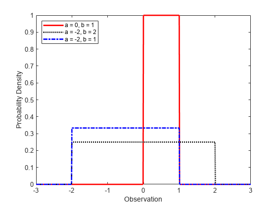
$f (x | a, b) = {\begin{matrix} (\frac{1}{b - a}); a \leq x \leq b \\ 0; o t h e r w i s e \end{matrix} .$

The pdf is constant between a and b.

For an example, see Compute Continuous Uniform Distribution pdf.

Cumulative Distribution Function

The cumulative distribution function (cdf) of the uniform distribution is

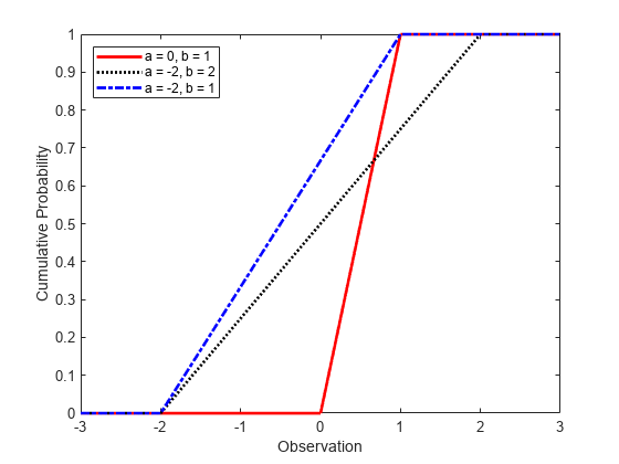
$F (x | a, b) = {\begin{matrix} 0; x < a \\ \frac{x - a}{b - a}; a \leq x < b \\ 1; x \geq b \end{matrix} .$

The result p is the probability that a single observation from a uniform distribution with parameters a and b falls in the interval [a x].

For an example, see Compute Continuous Uniform Distribution cdf.

Descriptive Statistics

The mean of the uniform distribution is $μ = \frac{1}{2} (a + b)$ .

The variance of the uniform distribution is $σ^{2} = \frac{1}{12} {(b - a)}^{2}$ .

Random Number Generation

You can use the standard uniform distribution to generate random numbers for any other continuous distribution by the inversion method. The inversion method relies on the principle that continuous cumulative distribution functions (cdfs) range uniformly over the open interval (0, 1). If u is a uniform random number on (0, 1), then x = F^–1(u) generates a random number x from the continuous distribution with the specified cdf F.

For an example, see Generate Random Numbers Using Uniform Distribution Inversion.

Examples

Compute Continuous Uniform Distribution pdf

Open Live Script

Create three uniform distribution objects with different parameters.

pd1 = makedist('Uniform');                      % Standard uniform distribution
pd2 = makedist('Uniform','lower',-2,'upper',2); % Uniform distribution with a = -2 and b = 2
pd3 = makedist('Uniform','lower',-2,'upper',1); % Uniform distribution with a = -2 and b = 1

Compute the pdfs for the three uniform distributions.

x = -3:.01:3;
pdf1 = pdf(pd1,x);
pdf2 = pdf(pd2,x);
pdf3 = pdf(pd3,x);

Plot the pdfs on the same axis.

figure;
plot(x,pdf1,'r','LineWidth',2); 
hold on;
plot(x,pdf2,'k:','LineWidth',2);
plot(x,pdf3,'b-.','LineWidth',2);
legend({'a = 0, b = 1','a = -2, b = 2','a = -2, b = 1'},'Location','northwest');
xlabel('Observation')
ylabel('Probability Density')
hold off;

Figure contains an axes object. The axes object with xlabel Observation, ylabel Probability Density contains 3 objects of type line. These objects represent a = 0, b = 1, a = -2, b = 2, a = -2, b = 1.

As the width of the interval (a,b) increases, the height of each pdf decreases.

Compute Continuous Uniform Distribution cdf

Open Live Script

Create three uniform distribution objects with different parameters.

pd1 = makedist('Uniform');                      % Standard uniform distribution
pd2 = makedist('Uniform','lower',-2,'upper',2); % Uniform distribution with a = -2 and b = 2
pd3 = makedist('Uniform','lower',-2,'upper',1); % Uniform distribution with a = -2 and b = 1

Compute the cdfs for the three uniform distributions.

x = -3:.01:3;
cdf1 = cdf(pd1,x);
cdf2 = cdf(pd2,x);
cdf3 = cdf(pd3,x);

Plot the cdfs on the same axis.

figure;
plot(x,cdf1,'r','LineWidth',2); 
hold on;
plot(x,cdf2,'k:','LineWidth',2);
plot(x,cdf3,'b-.','LineWidth',2);
legend({'a = 0, b = 1','a = -2, b = 2','a = -2, b = 1'},'Location','NW');
xlabel('Observation')
ylabel('Cumulative Probability')
hold off;

Figure contains an axes object. The axes object with xlabel Observation, ylabel Cumulative Probability contains 3 objects of type line. These objects represent a = 0, b = 1, a = -2, b = 2, a = -2, b = 1.

As the width of the interval (a,b) increases, the slope of each cdf decreases.

Related Distributions

Beta Distribution — The beta distribution is a two-parameter continuous distribution that has parameters a (first shape parameter) and b (second shape parameter). The standard uniform distribution is equal to the beta distribution with unit parameters.
Triangular Distribution — The triangular distribution is a three-parameter continuous distribution that has parameters a (lower limit), b (peak), and c (upper limit). The sum of two random variables with a standard uniform distribution has a triangular distribution with a = 0, b = 1, and c = 0.

References

[1] Abramowitz, Milton, and Irene A. Stegun, eds. Handbook of Mathematical Functions: With Formulas, Graphs, and Mathematical Tables. 9. Dover print.; [Nachdr. der Ausg. von 1972]. Dover Books on Mathematics. New York, NY: Dover Publ, 2013.

[2] Devroye, Luc. Non-Uniform Random Variate Generation. New York, NY: Springer New York, 1986. https://doi.org/10.1007/978-1-4613-8643-8

[3] Evans, Merran, Nicholas Hastings, and Brian Peacock. Statistical Distributions. 2nd ed. New York: J. Wiley, 1993.