Classify
Classify data using a trained deep learning neural network
Libraries:
Deep Learning Toolbox /
Deep Neural Networks
Description
The Classify block predicts class labels for the data at the input by using the trained network specified through the block parameter. This block allows loading of a pretrained network into the Simulink® model from a MAT file or from a MATLAB® function.
Examples
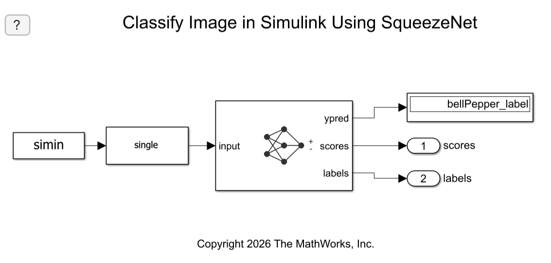
Classify Image in Simulink Using SqueezeNet
Classify an image in Simulink® using the Classify block.

Classify ECG Signals in Simulink Using Deep Learning
Use wavelet transforms and a deep learning network within a Simulink (R) model to classify ECG signals. This example uses the pretrained convolutional neural network from the Classify Time Series Using Wavelet Analysis and Deep Learning example of the Wavelet Toolbox™ to classify ECG signals based on images from the CWT of the time series data. For information on training, see Classify Time Series Using Wavelet Analysis and Deep Learning (Wavelet Toolbox).
Limitations
The Classify block does not support MAT file logging.
Ports
Input
A h-by-w-by-c-by-N numeric array, where h, w, and c are the height, width, and number of channels of the images, respectively, and N is the number of images.
A N-by-numFeatures numeric array, where
N is the number of observations and
numFeatures is the number of features of the input data.
If the array contains NaNs, then they are propagated through
the network.
Output
Predicted class labels with the highest score, returned as a N-by-1 enumerated vector of labels, where N is the number of observations.
Predicted scores, returned as a K-by-N matrix, where K is the number of classes, and N is the number of observations.
Labels associated with the predicted scores, returned as a N-by-K matrix, where N is the number of observations, and K is the number of classes.
Parameters
Specify the source for the trained network. Select one of the following:
Network from MAT file— Import a trained network from a MAT file containing adlnetworkobject.Network from MATLAB function— Import a pretrained network from a MATLAB function. For example, to use a pretrained GoogLeNet, create a functionpretrainedGoogLeNetin a MATLAB M-file, and then import this function.function net = pretrainedGoogLeNet net = imagePretrainedNetwork("googlenet"); end
Programmatic Use
Block Parameter:
Network |
| Type: character vector, string |
Values:
'Network from MAT file' | 'Network
from MATLAB function' |
Default:
'Network from MAT file' |
This parameter specifies the name of the MAT file that contains the trained deep learning network to load. If the file is not on the MATLAB path, use the Browse button to locate the file.
Dependencies
To enable this parameter, set the Network
parameter to Network from MAT
file.
Programmatic Use
Block Parameter:
NetworkFilePath |
| Type: character vector, string |
| Values: MAT file path or name |
Default:
'untitled.mat'
|
This parameter specifies the name of the MATLAB function for the pretrained deep learning
network. For example, to use a pretrained GoogLeNet, create a function
pretrainedGoogLeNet in a MATLAB M-file, and then import this
function.
function net = pretrainedGoogLeNet
  net = imagePretrainedNetwork("googlenet");
end
Dependencies
To enable this parameter, set the Network parameter to Network from MATLAB function.
Programmatic Use
Block Parameter: NetworkFunction |
| Type: character vector, string |
| Values: MATLAB function name |
Default: 'squeezenet' |
Size of mini-batches to use for prediction, specified as a positive integer. Larger mini-batch sizes require more memory, but can lead to faster predictions.
Programmatic Use
Block Parameter: MiniBatchSize |
| Type: character vector, string |
| Values: positive integer |
Default: '128' |
Resize the data at the input port to the input size of the network.
Programmatic Use
Block Parameter:
ResizeInput |
| Type: character vector, string |
Values:
'off' | 'on' |
Default:
'on' |
Since R2026a
Auto mode–– This option automatically selects the simulation mode based on the model configuration and code generation compatibility. It usesCode generationwhenever code generation is supported and switches toInterpreted executionwhen the model is incompatible for code generation.Interpreted execution–– Simulate model using the MATLAB interpreter. This option shortens startup time but has a slower simulation speed thanCode generation. In this mode, you can debug the source code of the block.Code generation–– Simulate model using generated code.The first time you simulate a model that contains a Classify block, the software generates binary code or C/C++ MATLAB executable (MEX) code from the block and integrates this code with the model. The Classify block uses the same infrastructure as MATLAB Coder™, which you use to generate C/C++ code from MATLAB code outside of Simulink. The generated code is reused for subsequent simulations, as long as the model does not change. This option requires additional startup time, but the speed of the subsequent simulations is comparable to
Interpreted execution.
If your Simulink model is set up to simulate in Normal mode and if you use Classify block via code generation, individual Classify blocks can take advantage of acceleration via code generation. If the Simulink model is set up to simulate in accelerator mode or any of the other target modes, Classify block's Simulate using parameter does not have any effect. However, there is one exception, if the model is set up to simulate in accelerator mode and you use Classify block with interpreted execution mode, the block will run in interpreted execution mode.
Programmatic Use
Block Parameter:
SimulateUsing |
| Type: character vector, string |
Values:
"Auto mode" | "Interpreted execution" |
"Code generation" |
Default:
"Auto mode" |
Enable output port ypred that outputs the label with the highest score.
Programmatic Use
Block Parameter: Classification |
| Type: character vector, string |
Values: 'off' | 'on' |
Default: 'on' |
Enable output ports scores and labels that output all predicted scores and associated class labels.
Programmatic Use
Block Parameter: Predictions |
| Type: character vector, string |
Values: 'off' | 'on' |
Default: 'off' |
Variable containing class names, specified as a categorical vector, a string array, or a cell array of character vectors.
The output size of the network must match the number of classes.
Dependencies
To enable this parameter, set the Network
parameter to Network from MAT file to
import a trained dlnetwork object
from a MAT file.
Programmatic Use
Block Parameter:
classNames |
| Type:variable name of a categorical vector, a string array, or a cell array of character vectors. |
| Values: Name of a variable containing class names, specified as a categorical vector, a string array, or a cell array of character vectors. |
Default: The workspace variable
classNames. |
Tips
You can accelerate your simulations with code generation taking advantage of the Intel® MKL-DNN library. For more details, see Acceleration for Simulink Deep Learning Models.
Extended Capabilities
Usage notes and limitations:
To generate generic C code that does not depend on third-party libraries, in the Configuration Parameters > Code Generation general category, set the Language parameter to
C.To generate C++ code, in the Configuration Parameters > Code Generation general category, set the Language parameter to
C++. To specify the target library for code generation, in the Code Generation > Interface category, set the Target Library parameter. Setting this parameter toNonegenerates generic C++ code that does not depend on third-party libraries.For a list of networks and layers supported for code generation, see Networks and Layers Supported for Code Generation (MATLAB Coder).
Usage notes and limitations:
The Language parameter in the Configuration Parameters > Code Generation general category must be set to
C++.For a list of networks and layers supported for CUDA® code generation, see Supported Networks, Layers, and Classes (GPU Coder).
To learn more about generating code for Simulink models containing the Classify block, see Code Generation for a Deep Learning Simulink Model to Classify ECG Signals (GPU Coder).
Version History
Introduced in R2020bIn R2026a, the Image Classifier block is renamed the Classify block, expanding its
capabilities beyond image-based classification. The Classify block
supports 1-D, 2-D, and 3-D spatial data, and spatiotemporal data.
Starting in R2024a, the SeriesNetwork and DAGNetwork
objects are not recommended. This recommendation means that SeriesNetwork
and DAGNetwork inputs to the Classify block are not
recommended. Use the dlnetwork objects instead.
dlnetwork objects have these advantages:
dlnetworkobjects are a unified data type that supports network building, prediction, built-in training, visualization, compression, verification, and custom training loops.dlnetworkobjects support a wider range of network architectures that you can create or import from external platforms.The
trainnetfunction supportsdlnetworkobjects, which enables you to easily specify loss functions. You can select from built-in loss functions or specify a custom loss function.Training and prediction with
dlnetworkobjects is typically faster thanLayerGraphandtrainNetworkworkflows.
Simulink block models with dlnetwork objects behave differently. The
predicted scores are returned as a K-by-N matrix, where K is the
number of classes, and N is the number of observations.
If you have an existing Simulink block model with a SeriesNetwork or
DAGNetwork object, follow these steps to use a dlnetwork object instead:
Convert the
SeriesNetworkorDAGNetworkobject to adlnetworkusing thedag2dlnetworkfunction.Define a workspace variable containing class names of the network output corresponding to the block parameter Class names workspace variable.
Transpose the predicted scores using a transpose block to an N-by-K array, where N is the number of observations, and K is the number of classes.
See Also
MATLAB Command
You clicked a link that corresponds to this MATLAB command:
Run the command by entering it in the MATLAB Command Window. Web browsers do not support MATLAB commands.
选择网站
选择网站以获取翻译的可用内容,以及查看当地活动和优惠。根据您的位置,我们建议您选择:。
您也可以从以下列表中选择网站:
如何获得最佳网站性能
选择中国网站(中文或英文)以获得最佳网站性能。其他 MathWorks 国家/地区网站并未针对您所在位置的访问进行优化。
美洲
- América Latina (Español)
- Canada (English)
- United States (English)
欧洲
- Belgium (English)
- Denmark (English)
- Deutschland (Deutsch)
- España (Español)
- Finland (English)
- France (Français)
- Ireland (English)
- Italia (Italiano)
- Luxembourg (English)
- Netherlands (English)
- Norway (English)
- Österreich (Deutsch)
- Portugal (English)
- Sweden (English)
- Switzerland
- United Kingdom (English)