Estimating Models Using Frequency-Domain Data
The System Identification Toolbox™ software lets you use frequency-domain data to identify linear models at the command line and in the System Identification app. You can estimate both continuous-time and discrete-time linear models using frequency-domain data. This topic presents an overview of model estimation in the toolbox using frequency-domain data. For an example of model estimation using frequency-domain data, see Frequency Domain Identification: Estimating Models Using Frequency Domain Data.
Frequency-domain data can be of two types:
Frequency domain input-output data — You obtain the data by computing Fourier transforms of time-domain input, u(t), and output, y(t), signals. The data is the set of input, U(ω), and output, Y(ω), signals in frequency domain. In the toolbox, frequency-domain input-output data is represented using
iddataobjects. For more information, see Representing Frequency-Domain Data in the Toolbox.Frequency-response data — Also called frequency function or frequency-response function (FRF), the data consists of transfer function measurements, G(iω), of a system at a discrete set of frequencies ω. Frequency-response data at a frequency ω tells you how a linear system responds to a sinusoidal input of the same frequency. In the toolbox, frequency-response data is represented using
idfrdobjects. For more information, see Representing Frequency-Domain Data in the Toolbox. You can obtain frequency-response data in the following ways:Measure the frequency-response data values directly, such as by using a spectrum analyzer.
Perform spectral analysis of time-domain or frequency-domain input-output data (
iddataobjects) using commands such asspaandspafdr.Compute the frequency-response of an identified linear model using commands such as
freqresp,bode, andidfrd.
The workflow for model estimation using frequency-domain data is the same as that for estimation using time-domain data. If needed, you first prepare the data for model identification by removing outliers and filtering the data. You then estimate a linear parametric model from the data, and validate the estimation.
Advantages of Using Frequency-Domain Data
Using frequency-domain data has the following advantages:
Data compression — You can compress long records of data when you convert time-domain data to frequency domain. For example, you can use logarithmically spaced frequencies.
Non uniformity — Frequency-domain data does not have to be uniformly spaced. Your data can have frequency-dependent resolution so that more data points are used in the frequency regions of interest. For example, the frequencies of interest could be the bandwidth range of a system, or near the resonances of a system.
Prefiltering — Prefiltering of data in the frequency-domain becomes simple. It corresponds to assigning different weights to different frequencies of the data.
Continuous-time signal - You can represent continuous-time signals using frequency-domain data and use the data for estimation.
Representing Frequency-Domain Data in the Toolbox
Before performing model estimation, you specify the frequency-domain data as objects in the toolbox. You can specify both continuous-time and discrete-time frequency-domain data.
Frequency domain input-output data — Specify as an
iddataobject. In the object, you store U(ω), Y(ω), and frequency vector ω. TheDomainproperty of the object is'Frequency', to specify that the object contains frequency-domain signals. If U(ω), Y(ω) are discrete-time Fourier transforms of discrete-time signals, sampled with sampling intervalTs, denote the sampling interval in theiddataobject. If U(ω), Y(ω) are Fourier transforms of continuous-time signals, specifyTsas0in theiddataobject.To plot the data at the command line, use the
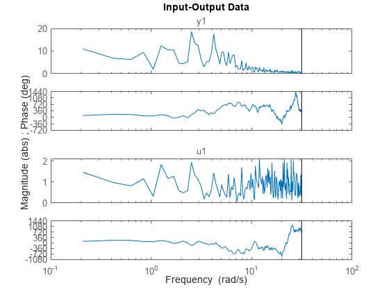
idplotcommand.For example, you can plot the phase and magnitude of frequency-domain input-output data.
Load time-domain input-output data.
load iddata1 z1
The time-domain inputs
uand outputsyare stored inz1, aniddataobject whoseDomainproperty is set to'Time'.Fourier-transform the data to obtain frequency-domain input-output data.
zf = fft(z1);
The
Domainproperty ofzfis set to'Frequency', indicating that it is frequency-domain data.Plot the magnitude and phase of the frequency-domain input-output data.
plot(zf)
Frequency-response data — Specify as an
idfrdobject. If you have Control System Toolbox™ software, you can also specify the data as anfrd(Control System Toolbox) object.To plot the data at the command line, use the
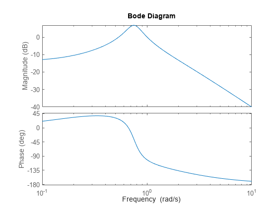
bodecommand.For example, you can plot the frequency-response of a transfer function model.
Create a transfer function model of your system.
sys = tf([1 0.2],[1 2 1 1]);
Calculate the frequency-response of the transfer function model,
sys, at 100 frequency points. Specify the range of the frequencies as 0.1 rad/s to 10 rad/s.freq = logspace(-1,1,100); frdModel = idfrd(sys,freq);
Plot the frequency-response of the model.
bode(frdModel)
For more information about the frequency-domain data types and how to specify them, see Frequency-Domain Data Representation.
You can also transform between frequency-domain and time-domain data types using the following commands.
| Original Data Format | To Time-Domain Data ( iddata object) | To Frequency-Domain Data ( iddata object) | To Frequency-Response Data ( idfrd object) |
|---|---|---|---|
| Time-Domain Data ( iddata object) | N/A | Use fft | |
| Frequency-Domain Data ( iddata object) | Use ifft (works only
for evenly spaced frequency-domain data). | N/A | |
| Frequency-Response Data ( idfrd object) | Not supported | Use iddata. The software
creates a frequency-domain iddata object that
has the same ratio between output and input as the original idfrd object
frequency-response data. |
|
For more information about transforming between data types in the app or at the command line, see the Transform Data category page.
Continuous-Time and Discrete-Time Frequency-Domain Data
Unlike time-domain data, the sample time Ts of
frequency-domain data can be zero. Frequency-domain data with zero Ts is
called continuous-time data. Frequency-domain data with Ts greater
than zero is called discrete-time data.
You can obtain continuous-time frequency-domain data
(Ts = 0) in the following ways:
Generate the data from known continuous-time analytical expressions.
For example, suppose that you know the frequency-response of your system is , where b is a constant. Also assume that the time-domain inputs to your system are, , where a is a constant greater than zero, and u(t) is zero for all times t less than zero. You can compute the Fourier transform of u(t) to obtain
Using U(ω) and G(ω) you can then get the frequency-domain expression for the outputs:
You can now evaluate the analytical expressions for Y(ω) and U(ω) over a grid of frequency values , and get a vector of frequency-domain input-output data values . You can package the input-output data as a continuous-time
iddataobject by specifying a zero sample time,Ts.Ts = 0; zf = iddata(Ygrid,Ugrid,Ts,'Frequency',wgrid)Compute the frequency response of a continuous-time linear system at a grid of frequencies.
For example, in the following code, you generate continuous-time frequency-response data,
FRDc, from a continuous-time transfer function model,sysfor a grid of frequencies,freq.sys = idtf(1,[1 2 2]); freq = logspace(-2,2,100); FRDc = idfrd(sys,freq);
Measure amplitudes and phases from a sinusoidal experiment, where the measurement system uses anti-aliasing filters. You measure the response of the system to sinusoidal inputs at different frequencies, and package the data as an
idfrdobject. For example, the frequency-response data measured with a spectrum analyzer is continuous-time.You can also conduct an experiment by using periodic, continuous-time signals (multiple sine waves) as inputs to your system and measuring the response of your system. Then you can package the input and output data as an
iddataobject.
You can obtain discrete-time frequency-domain data
(Ts >0) in the following ways:
Transform the measured time-domain values using a discrete Fourier transform.
For example, in the following code, you compute the discrete Fourier transform of time-domain data,
y, that is measured at discrete time-points with sample time 0.01 seconds.t = 0:0.01:10; y = iddata(sin(2*pi*10*t),[],0.01); Y = fft(y);
Compute the frequency response of a discrete-time linear system.
For example, in the following code, you generate discrete-time frequency-response data,
FRDd, from a discrete-time transfer function model,sys. You specify a non-zero sample time for creating the discrete-time model.Ts = 1; sys = idtf(1,[1 0.2 2.1],Ts); FRDd = idfrd(sys,logspace(-2,2,100));
You can use continuous-time frequency-domain data to identify only continuous-time models. You can use discrete-time frequency-domain data to identify both discrete-time and continuous-time models. However, identifying continuous-time models from discrete-time data requires knowledge of the intersample behavior of the data. For more information, see Estimating Continuous-Time and Discrete-Time Models.
Note
For discrete-time data, the software ignores frequency-domain data above the Nyquist frequency during estimation.
Preprocessing Frequency-Domain Data for Model Estimation
After you have represented your frequency-domain data using iddata or idfrd objects,
you can prepare the data for estimation by removing spurious data
and by filtering the data.
To view the spurious data, plot the data in the app, or use the idplot (for iddata objects) or bode (for idfrd objects) commands. After identifying the
spurious data in the plot, you can remove them. For example, if you want to remove data points
20–30 from zf, a frequency-domain iddata object, use the
following syntax:
zf(20:30) = [];
Since frequency-domain data does not have to be specified with a uniform spacing, you do not need to replace the outliers.
You can also prefilter high-frequency noise in your data. You
can prefilter frequency-domain data in the app, or use idfilt at the command line. Prefiltering
data can also help remove drifts that are low-frequency disturbances.
In addition to minimizing noise, prefiltering lets you focus your
model on specific frequency bands. The frequency range of interest
often corresponds to a passband over the breakpoints on a Bode plot.
For example, if you are modeling a plant for control-design applications,
you can prefilter the data to enhance frequencies around the desired
closed-loop bandwidth.
For more information, see Filtering Data.
Estimating Linear Parametric Models
After you have preprocessed the frequency-domain data, you can use it to estimate continuous-time and discrete-time models.
Supported Model Types
You can estimate the following linear parametric models using frequency-domain data. The noise component of the models is not estimated, except for ARX models.
| Model Type | Additional Information | Estimation Commands | Estimation in the App |
|---|---|---|---|
| Transfer Function Models | See Estimate Transfer Function Models in the System Identification App. | ||
| State-Space Models | Estimated K matrix of the state-space model
is zero. | See Estimate State-Space Models in System Identification App. | |
| Process Models | Disturbance model is not estimated. | See Estimate Process Models Using the App. | |
| Input-Output Polynomial Models | You can estimate only output-error and ARX models. | See Estimate Polynomial Models in the App. | |
| Linear Grey-Box Models | Model parameters that are only related to the noise matrix K are
not estimated. | Grey-box model estimation is not available in the app. | |
| Correlation Models (Impulse-response models) | See Estimate Impulse-Response Models Using System Identification App. | ||
| Frequency-Response Models (Estimated as idfrd objects) | See Estimate Frequency-Response Models in the App. |
Before performing the estimation, you can specify estimation
options, such as how the software treats initial conditions of the
estimation data. To do so at the command line, use the estimation
option set corresponding to the estimation command. For example, suppose
that you want to estimate a transfer function model from frequency-domain
data, zf, and you also want to estimate the initial
conditions of the data. Use the tfestOptions option
set to specify the estimation options, and then estimate the model.
opt = tfestOptions('InitialCondition','estimate');
sys = tfest(zf,opt);
sys is the estimated transfer function model.
For information about extracting estimated parameter values from the
model, see Extracting Numerical Model Data. After
performing the estimation, you can validate the estimated model.
Note
A zero initial condition for time-domain data does not imply a zero initial condition for the corresponding frequency-domain data. For time-domain data, zero initial conditions mean that the system is assumed to be in a state of rest before the start of data collection. In the frequency-domain, initial conditions can be ignored only if the data collected is periodic in nature. Thus, if you have time-domain data collected with zero initial conditions, and you convert it to frequency-domain data to estimate a model, you have to estimate the initial conditions as well. You cannot specify them as zero.
You cannot perform the following estimations using frequency-domain data:
Estimation of the noise component of a linear model, except for ARX models.
Estimation of time series models using spectrum data only. Spectrum data is the power spectrum of a signal, commonly stored in the
SpectrumDataproperty of anidfrdobject.
Estimating Continuous-Time and Discrete-Time Models
You can estimate all the supported linear models as discrete-time models, except for process models. Process models are defined in continuous-time only. For the estimation of discrete-time models, you must use discrete-time data.
You can estimate all the supported linear models as continuous-time
models, except for correlation models (see impulseest).
You can estimate continuous-time models using both continuous-time
and discrete-time data. For information about continuous-time and
discrete-time data, see Continuous-Time and Discrete-Time Frequency-Domain Data.
If you are estimating a continuous-time model using discrete-time data, you must specify the intersample behavior of the data. The specification of intersample behavior depends on the type of frequency-domain data.
Discrete-time frequency-domain input-output data (
iddataobject) — Specify the intersample behavior of the time-domain input signal u(t) that you Fourier transformed to obtain the frequency-domain input signal U(ω).Discrete-time frequency-response data (
idfrdobject) — The data is generated by computing the frequency-response of a discrete-time model. Specify the intersample behavior as the discretization method assumed to compute the discrete-time model from an underlying continuous-time model. For an example, see Specify Intersample Behavior for Discrete-Time Frequency-Response Data.
You can specify the intersample behavior to be piecewise constant (zero-order hold), linearly interpolated between the samples (first-order hold), or band-limited. If you specify the discrete-time data from your system as band-limited (that is no power above the Nyquist frequency), the software treats the data as continuous-time by setting the sample time to zero. The software then estimates a continuous-time model from the data. For more information, see Effect of Input Intersample Behavior on Continuous-Time Models.
Specify Intersample Behavior for Discrete-Time Frequency-Response Data
This example shows the effect of intersample behavior on the estimation of continuous-time models using discrete-time frequency-response data.
Generate discrete-time frequency-response data. To do so, first construct a continuous-time transfer function model, sys. Then convert it to a discrete-time model, sysd, using the c2d command and first-order hold (FOH) method. Use the discrete-time model sysd to generate frequency-response data at specified frequencies, freq.
sys = idtf([1 0.2],[1 2 1 1]);
sysd = c2d(sys,1,c2dOptions('Method','foh'));
freq = logspace(-1,0,10);
FRdata = idfrd(sysd,freq);
FRdata is discrete-time data. The software sets the InterSample property of FRdata to 'foh', which is the discretization method that was used to obtain sysd from sys.
Estimate a third-order continuous-time transfer function from the discrete-time data.
model1 = tfest(FRdata,3,1)
model1 =

        s + 0.2
  -------------------
  s^3 + 2 s^2 + s + 1

Continuous-time identified transfer function.

Parameterization:
   Number of poles: 3   Number of zeros: 1
   Number of free coefficients: 5
   Use "tfdata", "getpvec", "getcov" for parameters and their uncertainties.

Status:
Estimated using TFEST on frequency response data "FRdata".
Fit to estimation data: 100%
FPE: 7.11e-27, MSE: 2.375e-27

Model Properties
model1 is a continuous-time model, estimated using discrete-time frequency-response data. The underlying continuous-time dynamics of the original third-order model sys are retrieved in model1 because the correct intersample behavior is specified in FRdata.
Now, specify the intersample behavior as zero-order hold (ZOH), and estimate a third-order transfer function model.
FRdata.InterSample = 'zoh';
model2 = tfest(FRdata,3,1)
model2 =
-15.49 s - 3.307
---------------------------------
s^3 - 30.03 s^2 - 6.825 s - 17.04
Continuous-time identified transfer function.
Parameterization:
Number of poles: 3 Number of zeros: 1
Number of free coefficients: 5
Use "tfdata", "getpvec", "getcov" for parameters and their uncertainties.
Status:
Estimated using TFEST on frequency response data "FRdata".
Fit to estimation data: 94.71%
FPE: 0.004862, MSE: 0.001622
Model Properties
model2 does not capture the dynamics of the original model sys. Thus, sampling related errors are introduced in the model estimation when the intersample behavior is not correctly specified.
Convert Frequency-Response Data Model to a Transfer Function
This example shows how to convert a frequency-response data (FRD) model to a transfer function model. You treat the FRD model as estimation data and then estimate the transfer function.
Obtain an FRD model.
For example, use bode to obtain the magnitude and phase response data for the following fifth-order system:
Use 100 frequency points between 0.1 rad/s to 10 rad/s to obtain the FRD model. Use frd to create a frequency-response model object.
freq = logspace(-1,1,100);
sys0 = tf([1 0.2],[1 1  0.8  0.4  0.12  0.04]);
[mag,phase] = bode(sys0,freq);
frdModel = frd(mag.*exp(1j*phase*pi/180),freq);
Obtain the best third-order approximation to the system dynamics by estimating a transfer function with 3 zeros and 3 poles.
np = 3;
nz = 3;
sys = tfest(frdModel,np,nz);
sys is the estimated transfer function.
Compare the response of the FRD Model and the estimated transfer function model.
bode(frdModel,sys,freq(1:50));
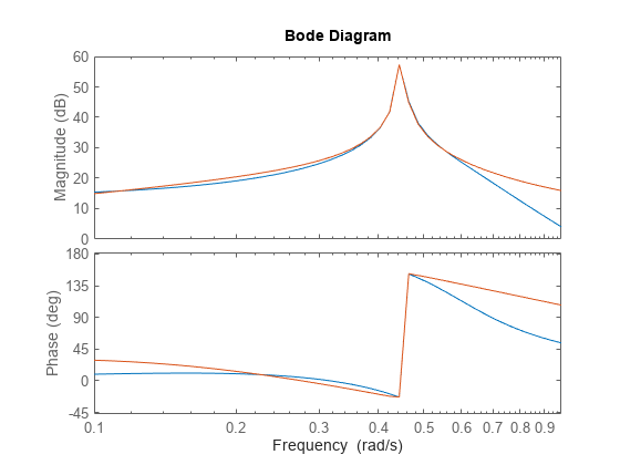
The FRD model is generated from the fifth-order system sys0. While sys, a third-order approximation, does not capture the entire response of sys0, it captures the response well until approximately 0.6 rad/s.
Validating Estimated Model
After estimating a model for your system, you can validate whether
it reproduces the system behavior within acceptable bounds. It is
recommended that you use separate data sets for estimating and validating
your model. You can use time-domain or frequency-domain data to validate
a model estimated using frequency-domain data. If you are using input-output
validation data to validate the estimated model, you can compare the
simulated model response to the measured validation data output. If
your validation data is frequency-response data, you can compare it
to the frequency response of the model. For example, to compare the
output of an estimated model sys to measured validation
data zv, use the following syntax:
compare(zv,sys);
You can also perform a residual analysis. For more information see, Validating Models After Estimation.
Troubleshooting Frequency-Domain Identification
When you estimate a model using frequency-domain data, the estimation
algorithm minimizes a loss (cost) function. For example, if you estimate
a SISO linear model from frequency-response data f,
the estimation algorithm minimizes the following least-squares loss
function:
Here, W is a frequency-dependent weight that you specify,
G is the linear model that is to be estimated, ω is the frequency, and
Nf is the number of frequencies at which the data
is available. The quantity is the frequency-response error. For frequency-domain input-output data, the
algorithm minimizes the weighted norm of the output error instead of the frequency-response
error. For more information, see Loss Function and Model Quality Metrics. During
estimation, spurious or uncaptured dynamics in your data can effect the loss function and
result in unsatisfactory model estimation.
Unexpected, spurious dynamics — Typically observed when the high magnitude regions of data have low signal-to-noise ratio. The fitting error around these portions of data has a large contribution to the loss function. As a result the estimation algorithm may overfit and assign unexpected dynamics to noise in these regions. To troubleshoot this issue:
Improve signal-to-noise ratio — You can gather more than one set of data, and average them. If you have frequency-domain input-output data, you can combine multiple data sets by using the
mergecommand. Use this data for estimation to obtain an improved result. Alternatively, you can filter the dataset, and use it for estimation. For example, use a moving-average filter over the data to smooth the measured response. Apply the smoothing filter only in regions of data where you are confident that the unsmoothness is due to noise, and not due to system dynamics.Reduce the impact of certain portions of data on the loss function — You can specify a frequency-dependent weight. For example, if you are estimating a transfer function model, specify the weight in the
WeightingFilteroption of the estimation option settfestOptions. Specify a small weight in frequency regions where the spurious dynamics exist. Alternatively, use fewer data points around this frequency region.
Uncaptured dynamics — Typically observed when the dynamics you want to capture have a low magnitude relative to the rest of data. Since a poor fit to low magnitude data contributes less to the loss function, the algorithm may ignore these dynamics to reduce errors at other frequencies. To troubleshoot this issue:
Specify a frequency-dependent weight — Specify a large weight for the frequency region where you would like to capture dynamics.
Use more data points around this region.
For an example of these troubleshooting techniques, see Troubleshoot Frequency-Domain Identification of Transfer Function Models.
If you do not achieve a satisfactory model using these troubleshooting techniques, try a different model structure or estimation algorithm.
Next Steps After Identifying a Model
After estimating a model, you can perform model transformations, extract model parameters, and simulate and predict the model response. Some of the tasks you can perform are:
Transforming Between Discrete-Time and Continuous-Time Representations
Transforming Between Linear Model Representations — Transform between linear parametric model representations, such as between polynomial, state-space, and zero-pole representations.
Extracting Numerical Model Data — For example, extract the poles and zeros of the model using
poleandzerocommands, respectively. Compute the model frequency response for a specified set of frequencies usingfreqresp.