主要内容

Data Sets for Signal Processing

R2026b
Since R2026a

Use these data sets with MATLAB® and Signal Processing Toolbox™ to get started with signal processing applications.

Audio and Acoustics Data Sets

Data SetData Set Information

Air Compressor

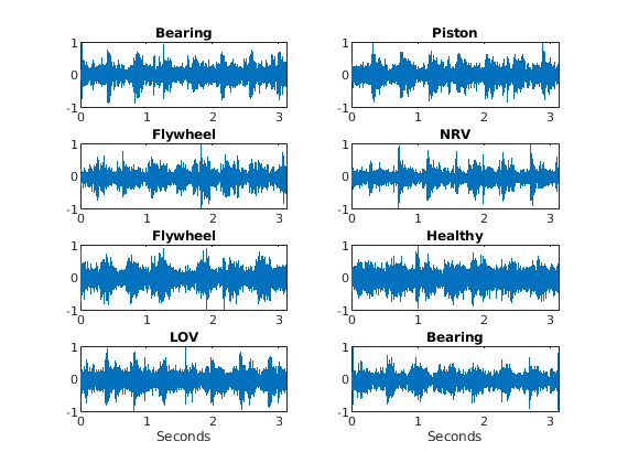
Air compressor data set. The figure shows eight signals in the time domain.

This data set comprises 1800 acoustic recordings collected on a single-stage reciprocating-type air compressor [1]. The data is collected at a sample rate of 16 kHz for 3.125 seconds.

The data set contains single-channel signals in eight subfolders that correspond to one of these operational states:

  • Healthy state — Normal compressor operation with no faults

  • Leakage inlet valve (LIV) fault — Fault in the inlet valve causing air leakage

  • Leakage outlet valve (LOV) fault — Fault in the outlet valve causing air leakage

  • Non-return valve (NRV) fault — Fault in the non-return valve preventing proper check valve operation

  • Piston ring fault — Worn or damaged piston rings affecting compression

  • Flywheel fault — Issues with the flywheel mechanism

  • Rider belt fault — Problems with the drive belt system

  • Bearing fault — Damaged or worn bearings causing vibration and noise

To learn more about this data set, expand these sections.

Download the data set programmatically.

url = "https://www.mathworks.com/supportfiles/audio/AirCompressorDataset/AirCompressorDataset.zip";
downloadFolder = fullfile(tempdir,"AirCompressorDataSet");
zipFile = fullfile(downloadFolder,"AirCompressorDataset.zip");
% Check if data set already exists. Otherwise, download it and unzip
if ~exist(fullfile(downloadFolder,"AirCompressorDataset"),"dir")
    if ~exist(downloadFolder,"dir")
        mkdir(downloadFolder);
    end
    websave(zipFile,url);
    unzip(zipFile,downloadFolder);
end

Load the signal data.

% Create audioDatastore object to manage audio files
datasetLocation = fullfile(tempdir,"AirCompressorDataSet","AirCompressorDataset");
ads = audioDatastore(datasetLocation,IncludeSubfolders=true,LabelSource="foldernames");
% Display data set information
fprintf("Total number of files: %d\n",numel(ads.Files));
fprintf("Class distribution:\n");
countEachLabel(ads)

Read and preview one sample.

[audioIn, info] = read(ads);
% Display sample information
fprintf("Sample information:\n");
fprintf("Filename: %s\n", info.FileName);
fprintf("Sample rate: %d Hz\n", info.SampleRate);
fprintf("Number of samples: %d\n", length(audioIn));
fprintf("Duration: %.4f seconds\n", length(audioIn)/info.SampleRate);
fprintf("Label: %s\n", string(info.Label));
% Reset datastore to beginning
reset(ads);

Structure:

AirCompressorDataset/
├── license.txt
├── Healthy/
│   ├── preprocess_Reading1.wav
│   ├── preprocess_Reading2.wav
│   └── ... (225 files total)
├── LIV/                    (Leakage Inlet Valve)
│   └── ... (225 files)
├── LOV/                    (Leakage Outlet Valve)
│   └── ... (225 files)
├── NRV/                    (Non-Return Valve)
│   └── ... (225 files)
├── Piston/                 (Piston Ring fault)
│   └── ... (225 files)
├── Flywheel/
│   └── ... (225 files)
├── Riderbelt/              (Rider Belt fault)
│   └── ... (225 files)
└── Bearing/                (Bearing fault)
    └── ... (225 files)

File details:

  • Size:

    • ZIP file: 163 MB

    • Extracted folder: 177 MB

    • Signal data (each WAV file): 97.7 KB

  • Signals: 1800 WAV files (8 subfolders of 225 WAV files)

  • Audio channels: 1 (mono)

  • Labels: Derived from subfolder names representing operational states.

  • Equipment specifications:

    • Air pressure range: 0-500 lb/m2, 0-35 Kg/cm2.

    • Induction motor: 5 HP, 415 V, 5 A, 50 Hz, 1440 RPM.

    • Pressure switch: Type PR-15, Range 100-213 PSI.

Phonocardiogram (PCG) Data — PhysioNet Challenge 2016

Phonocardiogram data set. The figure shows four signals in the time domain.

This data set comprises 3,829 acoustic recordings of heart sounds from the PhysioNet Computing in Cardiology Challenge 2016 [2][3]. The data is collected at a sample rate of 2 kHz for 5 seconds.

The data set supports binary classification of cardiac health status through automated phonocardiogram interpretation in resource-limited settings, remote cardiac health screening, and early detection of heart conditions.

  • Normal (2,575 recordings) — Persons with normal cardiac function, representing healthy heart sound patterns and reference baseline.

  • Abnormal (1,254 recordings) — Persons with abnormal cardiac function including various cardiac abnormalities, murmurs, valve disorders, and other pathologies.

Applications include automated cardiac screening systems, telemedicine and remote diagnostics, point-of-care cardiac assessment, medical training and education, and algorithm development for cardiac sound analysis.

To learn more about this data set, expand these sections.

Download the data set programmatically.

% Download from GitHub (manual download required)
% 1. Visit: https://github.com/mathworks/physionet_phonocardiogram
% 2. Click "Code" → "Download ZIP"
% 3. Extract physionet_phonocardiogram-main.zip

% Or use automated download:
githubUrl = "https://github.com/mathworks/physionet_phonocardiogram/archive/refs/heads/main.zip";
downloadFolder = fullfile(tempdir,"PhonCardioGram");
mainZipFile = fullfile(downloadFolder,"physionet_phonocardiogram-main.zip");
% Check if data set already exists, if not download and unzip
if ~exist(fullfile(downloadFolder,"PCG_Data"),"dir")
    if ~exist(downloadFolder,"dir")
        mkdir(downloadFolder);
    end
    % Download main repository
    websave(mainZipFile,githubUrl);
    unzip(mainZipFile,downloadFolder);
    % Extract PCG_Data.zip from within the repository
    pcgDataZip = fullfile(downloadFolder, ...
        "physionet_phonocardiogram-main","PCG_Data.zip");
    unzip(pcgDataZip,fullfile(downloadFolder,"PCG_Data"));
end

Load the signal data.

% Load the heart sound data
dataPath = fullfile(tempdir,"PhonCardioGram","PCG_Data","heartSoundData.mat");
load(dataPath);
% Display data set information
fprintf("Total recordings: %d\n",size(heartSoundData.Data,2));
fprintf("Samples per recording: %d\n",size(heartSoundData.Data,1));
fprintf("Duration per recording: %.1f seconds\n",size(heartSoundData.Data,1)/2000);
% Display class distribution
fprintf("Class distribution:\n");
summary(heartSoundData.Classes)

Read and preview one sample.

% Plot 2-by-2 grid, comparing normal and abnormal heart sounds
fs = 2000; % Sample rate in Hz
sampleIndices = [7 2 9 3]; % two normal, two abnormal
figure;
t = tiledlayout(2, 2);
for i = 1:4
    idx = sampleIndices(i);
    signal = heartSoundData.Data(:,idx);
    label = heartSoundData.Classes(idx);
    time = (0:length(signal)-1)/fs;
    nexttile;
    plot(time,signal)
    title("Sample " + idx + " (" + string(label) + ")")
    xlabel("Time (s)")
    ylabel("Amplitude")
    box on
    grid on
end
title(t,"PhonocardiogramData - Heart Sound Recordings")

Structure:

physionet_phonocardiogram-main/
├── heartSoundData.mat          (Primary data set - 69 MB)
│   ├── Data: [10000×3829 double]
│   └── Classes: [3829×1 categorical]
├── extrafiles.mat              (2.4 KB - source attributions)
├── Modified_physionet_data.txt (Attribution documentation)
├── License.txt
└── README.md

File details:

  • Size:

    • ZIP file: 68 MB

    • Extracted folder: ~137 MB

    • Main data (heartSoundData.mat file): 69 MB

  • Data matrix: 10,000 × 3,829 double (samples × recordings)

  • Labels: 3,829 × 1 categorical array ("normal" or "abnormal")

  • Storage format: Double-precision floating-point

  • The number of recordings between people with normal cardiac function (2,575 recordings or 67.25%) and with abnormal cardiac function (1,254 recordings or 32.75%) follow a class imbalance ratio of approximately 2:1.

  • A recommended data split of 70% training and 30% testing enables robust model development while maintaining sufficient test samples for evaluation.

Acoustic scenes — Detection and Classification of Acoustic Scenes (DCASE) 2013 Challenge

Acoustic-scene DCASE data set. The figure shows two signals in the time domain.

This data set comprises 200 environmental audio recordings from the Detection and Classification of Acoustic Scenes and Events (DCASE) 2013 challenge [4][5]. Each recording is collected at a sample rate of 44.1 kHz for 30 seconds.

The data set contains two-channel signals in two subfolders, comprising training data and test data.

  • The training and test sets consist of 100 training waveforms and 100 test waveforms recorded in 10 different environments: bus, busy street, office, open-air market, park, quiet street, restaurant, supermarket, tube, and tube station.

  • This data set supports acoustic scene classification for environmental sound recognition. Supported applications include smart city monitoring and urban planning, environmental noise assessment, context-aware mobile applications, acoustic event detection systems, audio surveillance and security, and assistive listening devices.

To learn more about this data set, expand these sections.

Download the data set programmatically.

dataUrl = "https://ssd.mathworks.com/supportfiles/WA/data/DCASE2013.zip";
downloadFolder = fullfile(tempdir,"DCASE2013");
zipFile = fullfile(downloadFolder,"DCASE2013.zip");
% Check if data set already exists. Otherwise, download it and unzip
if ~exist(fullfile(downloadFolder,"scenes_stereo"),"dir")
    if ~exist(downloadFolder,"dir")
        mkdir(downloadFolder);
    end
    % Download data set
    websave(zipFile,dataUrl);
    unzip(zipFile,downloadFolder);
end

Load the signal data.

% Create audioDatastore to manage the audio files
datasetLocation = fullfile(tempdir,"DCASE2013");
% Extract labels from file names and create training datastore
trainlabels = filenames2labels(fullfile(datasetLocation,"scenes_stereo"), ...
    ExtractBefore=digitsPattern);
adsTrain = audioDatastore(fullfile(datasetLocation,"scenes_stereo"), ...
    OutputDataType="single");
adsTrain.Labels = trainlabels;
% Extract labels from file names and create test datastore
testlabels = filenames2labels( ...
    fullfile(datasetLocation,"scenes_stereo_testset"),ExtractBefore=digitsPattern);
adsTest = audioDatastore( ...
    fullfile(datasetLocation,"scenes_stereo_testset"),OutputDataType="single");
adsTest.Labels = testlabels;
% Display data set information
fprintf("Training files: %d\n",numel(adsTrain.Files));
fprintf("Test files: %d\n",numel(adsTest.Files));
fprintf("Scene categories: %d\n",numel(categories(adsTrain.Labels)));
% Display label distribution
fprintf("\nTraining label distribution:\n");
countEachLabel(adsTrain)
fprintf("\nTest label distribution:\n");
countEachLabel(adsTest)

Read and preview one sample.

% Read one audio recording
[audio, info] = read(adsTrain);
fs = info.SampleRate;
% Display sample information
fprintf("Sample information:\n");
fprintf("  Filename: %s\n",info.FileName);
fprintf("  Sample rate: %d Hz\n",fs);
fprintf("  Number of channels: %d\n",size(audio,2));
fprintf("  Total samples: %d\n",size(audio,1));
fprintf("  Duration: %.2f seconds\n",size(audio,1)/fs);
% Reset datastore to beginning
reset(adsTrain);
% Plot both stereo channels
figure;
t = tiledlayout(2,1);
time = (0:size(audio,1)-1)/fs;
nexttile;
plot(time, audio(:,1))
ylabel("Left Channel")
box on
grid on
nexttile;
plot(time,audio(:,2))
xlabel("Time (s)")
ylabel("Right Channel")
box on
grid on
[~, fname, ~] = fileparts(info.FileName);
title(t,"DCASE2013 - " + fname)

Structure:

DCASE2013/
├── scenes_stereo/              (Training set - 100 files, flat structure)
│   ├── bus01.wav
│   ├── bus02.wav
│   ├── ...
│   ├── bus10.wav
│   ├── busystreet01.wav
│   ├── busystreet02.wav
│   ├── ...
│   ├── office01.wav
│   ├── openairmarket01.wav
│   ├── park01.wav
│   ├── quietstreet01.wav
│   ├── restaurant01.wav
│   ├── supermarket01.wav
│   ├── tube01.wav
│   └── tubestation01.wav
└── scenes_stereo_testset/      (Test set - 100 files, flat structure)
    ├── bus01.wav
    ├── bus02.wav
    ├── ...
    ├── busystreet01.wav
    ├── office01.wav
    ├── openairmarket01.wav
    ├── park01.wav
    ├── quietstreet01.wav
    ├── restaurant01.wav
    ├── supermarket01.wav
    ├── tube01.wav
    └── tubestation01.wav

Naming convention:

  • Format: {sceneType}{number}.wav

    • {sceneType} —Scene type, which has any of these values: bus, busystreet, office, openairmarket, park, quietstreet, restaurant, supermarket, tube, or tubestation.

    • {number} — Scene number, which ranges from 01 to 10 for each scene type

  • The labels must be extracted from the file names, not from the folder structure.

File details:

  • Size:

    • ZIP file: 707 MB

    • Extracted folder: ~0.99 GB

    • Signal data (each WAV file): ~3.5 MB (30 seconds, stereo)

  • Total files: 200 WAV files (100 training + 100 test)

  • Scene classes: 10 categories

  • Files per class: 20 (10 training + 10 test)

  • Audio format: WAV (stereo)

  • Sample rate: 44,100 Hz

  • Bit depth: 16-bit

  • Channels: 2 (stereo)

  • Duration: 30 seconds per file

  • Balanced data set: Equal representation across all scenes

Free Spoken Digits

Free spoken digits data set. The figure shows 10 signals in the time domain.

This data set comprises 2000 voice recordings of spoken digits (0-9) by four individuals [6]. Each recording is collected at a sample rate of 8 kHz for a variable duration from 0.14 to 2.28 seconds.

The data set contains 16-bit single-channel signals distributed in 200 recordings per spoken digit. The multiple speakers provide diversity in accents and vocal characteristics, supporting development of robust digit recognition systems that generalize across different voices.

To learn more about this data set, expand these sections.

Download the data set programmatically.

dataUrl = "https://ssd.mathworks.com/supportfiles/audio/FSDD.zip";
downloadFolder = fullfile(tempdir,"FSDD");
zipFile = fullfile(downloadFolder,"FSDD.zip");
% Check if data set already exists. Otherwise, download it and unzip
if ~exist(fullfile(downloadFolder),"dir")
    if ~exist(downloadFolder,"dir")
        mkdir(downloadFolder);
    end
    % Download data set
    websave(zipFile,dataUrl);
    unzip(zipFile,downloadFolder);
end

Load the signal data.

% Create audioDatastore to manage the audio files
datasetLocation = fullfile(tempdir,"FSDD","FSDD","recordings");
% Extract labels from filenames (digit is before first underscore)
labels = filenames2labels(datasetLocation,ExtractBefore="_");
ads = audioDatastore(datasetLocation);
ads.Labels = labels;
% % Display data set information
fprintf("Total recordings: %d\n",numel(ads.Files));
fprintf("Digit classes: %d (0-9)\n",numel(categories(ads.Labels)));
% Display label distribution
fprintf("\nLabel distribution:\n");
countEachLabel(ads)

Read and preview one sample.

% Find first sample of each digit (0-9)
digitIndices = zeros(1,10);
for d = 0:9
    idx = find(ads.Labels == string(d),1);
    digitIndices(d+1) = idx;
end
% Plot 2-by-5 grid showing one sample per digit
figure;
t = tiledlayout(2,5);
for d = 0:9
    idx = digitIndices(d+1);
    [audio,fs] = audioread(ads.Files{idx});
    time = (0:length(audio)-1)/fs;
    nexttile;
    plot(time,audio)
    title("Digit " + d)
    xlabel("Time (s)")
    ylabel("Amplitude")
    box on
    grid on
end
title(t,"FSDD: Spoken Digits (0-9)")

Structure:

FSDD/
├── recordings/                  (2,000 WAV files)
│   ├── 0_jackson_0.wav
│   ├── 0_jackson_1.wav
│   ├── ...
│   ├── 9_yweweler_49.wav
│   └── ...
└── license.txt

Naming convention:

  • Format: {digit}_{speaker}_{repetition}.wav

    • {digit} — Digit, which ranges from 0 to 9.

    • {speaker} — Speaker name, which has any of these values: jackson, nicolas, theo, or yweweler.

    • {repetition} — Recording sequential identification number, which ranges from 0 to 49.

  • Example: The 7_jackson_23.wav file contains the recording of the digit-7 pronunciation that Jackson spoke for the 24th time.

File details:

  • Size:

    • ZIP file: 9 MB

    • Extracted folder: ~10 MB

    • Signal data (each WAV file): between 3 and 20 KB

  • Classes: 10 (from 0 to 9)

  • Speakers: Four individuals

  • Speaker distribution: 500 recordings per speaker (50 per digit)

Mozilla.org® Common Voice Speech Denoising

Common Voice Speech Denoising data set. The figure shows four signals in the time domain.

This data set comprises 2800 speech recordings as a curated subset of Mozilla.org Common Voice open-source speech corpus [7]. Each recording is collected at a sample rate of 48 kHz for a variable duration from 2 to 10 seconds.

The data consists of 16-bit single-channel signals distributed in three subfolders: training, validation, and test.

  • The recordings contain read sentences from diverse text sources with varied vocabulary and sentence structures, capturing natural prosody and complete utterances from multiple diverse speakers across different genders, age groups (18-80+ years), English dialects, and recording quality levels.

  • The data enables development of speech enhancement systems that handle various noise scenarios, including environmental noise, electronic noise, and signal distortions. The clean speech serves as reference, with noise augmentation that can be applied to create noisy versions for signal processing applications.

To learn more about this data set, expand these sections.

Download the data set programmatically.

dataUrl = "https://ssd.mathworks.com/supportfiles/audio/commonvoice.zip";
downloadFolder = fullfile(tempdir,"CommonVoice");
zipFile = fullfile(downloadFolder,"commonvoice.zip");
% Check if data set already exists. Otherwise, download it and unzip
if ~exist(fullfile(downloadFolder,"commonvoice"),"dir")
    if ~exist(downloadFolder,"dir")
        mkdir(downloadFolder);
    end
    % Download data set
    websave(zipFile,dataUrl);
    unzip(zipFile,downloadFolder);
end

Load the signal data.

% Create audioDatastore for each data split
datasetLocation = fullfile(tempdir,"CommonVoice","commonvoice");
% Note: Files are located in clips/ subfolders within each split
trainFolder = fullfile(datasetLocation,"train","clips");
valFolder = fullfile(datasetLocation,"validation","clips");
testFolder = fullfile(datasetLocation,"test","clips");
% Training datastore
ads_train = audioDatastore(trainFolder, ...
    IncludeSubfolders=true, ...
    FileExtensions=".wav");
% Validation datastore
ads_val = audioDatastore(valFolder, ...
    IncludeSubfolders=true, ...
    FileExtensions=".wav");
% Test datastore
ads_test = audioDatastore(testFolder, ...
    IncludeSubfolders=true, ...
    FileExtensions=".wav");
% Display data set information
fprintf("Data set Information:\n");
fprintf("  Training files: %d\n",numel(ads_train.Files));
fprintf("  Validation files: %d\n",numel(ads_val.Files));
fprintf("  Test files: %d\n",numel(ads_test.Files));
fprintf("  Total files: %d\n", ...
    numel(ads_train.Files) + numel(ads_val.Files) + numel(ads_test.Files));
% Calculate total duration (approximate)
totalFiles = numel(ads_train.Files) + numel(ads_val.Files) + numel(ads_test.Files);
avgDuration = 5; % Approximate average duration in seconds
totalDuration = totalFiles*avgDuration;
fprintf("  Estimated total duration: %.1f hours\n",totalDuration/3600);

Read and preview one sample.

% Preview one speech sample
[audio,info] = read(ads_train);
reset(ads_train);
% Display sample information
fprintf("Speech Sample Information:\n");
fprintf("  Filename: %s\n",info.FileName);
fprintf("  Sample rate: %d Hz\n",info.SampleRate);
fprintf("  Duration: %.2f seconds\n",length(audio)/info.SampleRate);
fprintf("  Number of channels: %d\n",size(audio,2));
fprintf("  Total samples: %d\n",length(audio));
fprintf("  Data type: %s\n",class(audio));

Structure:

CommonVoice/
└── commonvoice/
    ├── train/
    │   └── clips/                  (~2,000 WAV files)
    │       ├── speaker01_001.wav
    │       ├── speaker01_002.wav
    │       └── ...
    ├── validation/
    │   └── clips/                  (~400 WAV files)
    │       ├── speaker50_001.wav
    │       └── ...
    ├── test/
    │   └── clips/                  (~400 WAV files)
    │       ├── speaker75_001.wav
    │       └── ...
    └── README.txt

File details:

  • Size:

    • ZIP file: 955 MB

    • Extracted folder: ~1 GB

    • Signal data (each WAV file): ~50-500KB (variable duration)

  • Total Files: 2,800, distributed in three sets:

    • Training: ~2,000 files (~71%)

    • Validation: ~400 files (~14%)

    • Test: ~400 files (~14%)

  • Audio Specifications:

    • Format: WAV (uncompressed PCM)

    • Bit depth: 16-bit signed integer

    • Channels: 1 (mono)

    • Average file size: ~200 KB

  • Speaker Diversity:

    • Gender distribution: Mixed (approximately balanced)

    • Age range: 18-80+ years

    • Accents: North American (US, Canadian), British (UK, Irish), and other English varieties

    • Recording conditions: Home recordings (varied quality)

  • Data Split Strategy:

    • Speaker-independent: Different speakers in train/val/test

    • Stratified: Balanced gender and accent distribution

    • Random sampling: Representative subset from larger corpus

  • Utterance Characteristics:

    • Sentence length: 5-20 words typically

    • Content: Read text from diverse sources

    • Speaking style: Natural reading pace

    • Quality: Generally high SNR in original recordings

Biomedical Data Sets

Data SetData Set Information

Electrocardiogram (ECG) Data — QT Wave

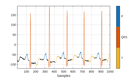
QT-wave electrocardiogram data set. The figure shows eight signals in the time domain.

This data set comprises 210 ECG recordings from 105 patients for automated waveform segmentation [2][8]. To obtain each recording, examiners placed two electrodes on different locations on a patient's chest and collected ECG waveforms at a sample rate of 250 Hz for approximately 15 minutes.

The data set contains two-channel ECG signals and four labeled cardiac regions:

  • P wave (atrial depolarization, <20 Hz frequency band)

  • QRS complex (ventricular depolarization, 10-40 Hz frequency band, most prominent ECG feature)

  • T wave (ventricular repolarization, <10 Hz frequency band)

  • N/A (unlabeled baseline and isoelectric segments)

The segmentation of these regions can provide the basis for measurements useful for assessing the overall health of the human heart and the presence of abnormalities [9].

To learn more about this data set, expand these sections.

Download the data set programmatically.

% Download and extract the QT Database ECG data set
dataUrl = "https://www.mathworks.com/supportfiles/SPT/data/QTDatabaseECGData.zip";
downloadFolder = fullfile(tempdir,"QTDatabaseECG");
zipFile = fullfile(downloadFolder,"QTDatabaseECGData.zip");
% Check if data set already exists. Otherwise, download it and unzip
if ~exist(fullfile(downloadFolder,"QTDataset"),"dir")
    if ~exist(downloadFolder,"dir")
        mkdir(downloadFolder);
    end
    % Download data set
    websave(zipFile,dataUrl);
    unzip(zipFile,downloadFolder);
end

Load the signal data.

% Create signalDatastore to manage the ECG data files
datasetLocation = fullfile(tempdir,"QTDatabaseECG","QTDataset");
sds = signalDatastore(datasetLocation, ...
    SignalVariableNames=["ecgSignal","signalRegionLabels"]);
% Display data set information
fprintf("Total number of ECG files: %d\n",numel(sds.Files));

Read and preview one sample.

% Read one ECG recording
[data,info] = read(sds);
% Extract signal and labels
ecgSignal = data{1};
regionLabels = data{2};
% Display sample information
fprintf("Sample information:\n");
fprintf("  Filename: %s\n",info.FileName);
fprintf("  Signal length: %d samples\n",length(ecgSignal));
fprintf("  Duration: %.2f seconds\n",length(ecgSignal)/250);
fprintf("  Number of labeled regions: %d\n",height(regionLabels));
% Display label information (first 10 rows)
fprintf("\nRegion labels (first 10 rows):\n");
disp(regionLabels(1:10,:));
% Display first few signal values
fprintf("\nFirst 10 signal values:\n");
disp(ecgSignal(1:10));
% Reset datastore
reset(sds);

Structure:

QTDataset/
├── License.txt
├── Modified_physionet_data.txt
├── ecg1.mat (ecgSignal, signalRegionLabels)
├── ecg2.mat
├── ecg3.mat
└── ... (210 MAT files total)

File details:

  • Size:

    • ZIP file: 44 MB

    • Extracted folder: ~45 MB

    • Signal data (each MAT file): ~200-220 KB

  • Total files: 210 MAT files

  • Patients: 105 participants

  • Channels per patient: 2 ECG leads, labeled separately

  • Variables per file: 2 (ecgSignal, signalRegionLabels)

  • Signal length: ~225,000 samples in double precision per file

  • Duration: ~15 minutes per recording

  • Processing segments: 5,000-sample windows (20 seconds each)

  • Label format: Table with region indices and categorical labels (P, QRS, T, N/A)

  • Total recording time: ~1,575 minutes (105 patients × 15 minutes)

  • Signal characteristics include baseline wander from respiratory motion occurring below 0.5 Hz, which affects ECG interpretation.

  • The noise components from respiratory motion present realistic challenges for automated analysis systems.

Myoelectric (EMG) Data — Arm motion

Arm-motion myoelectric data set. The figure shows eight signals in the time domain.

This data set comprises 720 EMG signal recordings measuring electrical muscle activity from 30 subjects performing various arm movements [10]. Each recording captured 3 seconds of motion at a sample rate of 3 kHz.

The data set contains 720 files with eight-channel EMG signals and 720 label files.

  • The recordings were collected across 4 sessions with 6 trials per session using with sensors placed on the subjects' forearm muscles to detect muscle activation pattern.

  • The label data includes seven motion categories: hand open, hand close, wrist flexion, wrist extension, supination, pronation, and rest. The motion arrays in each label file mark the forearm movements with numeric values from 1 to 6, and the rest periods have a mark of –1.

  • The multi-channel EMG configuration enables capture of complex muscle activation patterns across the forearm during different movements.

To learn more about this data set, expand these sections.

Download the data set programmatically.

dataUrl = "https://ssd.mathworks.com/supportfiles/SPT/data/MyoelectricData.zip";
downloadFolder = fullfile(tempdir,"MyoelectricData");
zipFile = fullfile(downloadFolder,"MyoelectricData.zip");
% Check if data set already exists. Otherwise, download it and unzip
if ~exist(fullfile(downloadFolder,"Data"),"dir")
    if ~exist(downloadFolder,"dir")
        mkdir(downloadFolder);
    end
    % Download data set
    websave(zipFile,dataUrl);
    unzip(zipFile,downloadFolder);
end

Load the signal data.

% Create signalDatastore for signal and label files
datasetLocation = fullfile(tempdir,"MyoelectricData","Data");
fs = 3000; % Sample rate in Hz
% Create datastore for signal files (ending with "d.mat")
sds1 = signalDatastore(datasetLocation, ...
    IncludeSubfolders=true, ...
    SampleRate=fs);
p = endsWith(sds1.Files,"d.mat");
sdssig = subset(sds1,p);
% Create datastore for label files (ending with "i.mat")
sds2 = signalDatastore(datasetLocation, ...
    SignalVariableNames=["motion";"data_indx"], ...
    IncludeSubfolders=true);
p = endsWith(sds2.Files,"i.mat");
sdslbl = subset(sds2,p);
% Display data set information
fprintf("Total signal files: %d\n",numel(sdssig.Files));
fprintf("Total label files: %d\n",numel(sdslbl.Files));

Read and preview one sample.

% Preview one EMG signal
signal = preview(sdssig);
% Display sample information
fprintf("Sample information:\n");
fprintf("  Number of channels: %d\n",size(signal,2));
fprintf("  Number of samples: %d\n",size(signal,1));
fprintf("  Duration: %.2f seconds\n",size(signal,1)/fs);
fprintf("  Sample rate: %d Hz\n",fs);
% Plot all channels to visualize muscle activation during one trial
figure;
t = tiledlayout(4,2);
for i = 1:8
    nexttile;
    plot(signal(:,i))
    title("Channel " + i)
    ylim([-1 1])
    box on
    grid on
end
[~,fname,~] = fileparts(sdssig.Files{1});
title(t,"MyoelectricData - " + fname)

Structure:

Data/
├── N01/
│   ├── N01S1/
│   │   ├── N01S1T1d.mat (EMG signal data - 8 channels)
│   │   ├── N01S1T1i.mat (motion labels)
│   │   ├── N01S1T2d.mat
│   │   ├── N01S1T2i.mat
│   │   ├── N01S1T3d.mat
│   │   ├── N01S1T3i.mat
│   │   ├── N01S1T4d.mat
│   │   ├── N01S1T4i.mat
│   │   ├── N01S1T5d.mat
│   │   ├── N01S1T5i.mat
│   │   ├── N01S1T6d.mat
│   │   └── N01S1T6i.mat (6 trials × 2 files = 12 files)
│   ├── N01S2/
│   │   └── ... (12 files)
│   ├── N01S3/
│   │   └── ... (12 files)
│   └── N01S4/
│       └── ... (12 files)
├── N02/
│   └── ... (4 sessions × 12 files = 48 files)
├── N03/
│   └── ... (48 files)
└── ... (N04 through N30)

File details:

  • Size:

    • ZIP file: 2.2 GB

    • Extracted folder: ~2.2 GB

    • Signal data (each MAT file): ~1.5 MB

  • Total files: 1,440 MAT files

    • Signal files: 720 (ending with d.mat)

    • Label files: 720 (ending with i.mat)

  • Files per subject: 48 files (24 signal + 24 label)

  • Subjects: 30 participants

  • Sessions per subject: 4

  • Trials per session: 6

  • Signal variables: Multi-channel EMG data (8 channels)

  • Label variables: Motion class indices (1-6) with rest periods (-1)

  • Channels: 8 EMG sensors

  • Motion duration: 3 seconds per motion

  • Repetitions: 4 per motion per trial

  • Total motion classes: 7 (6 arm motions + rest)

ECG Data — PhysioNet MIT-BIH

PhysioNet MIT-BIH ECG data set. The figure shows two signals in the time domain.

This data set comprises 46,080 segments of ECG signals and noise specifically prepared for ECG signal denoising applications. The recording captured 43.5 hours of ECG data from 47 subjects at a sample rate of 300 Hz. Each segment has 1024 samples, covering approximately 3.4 seconds of data.

The data set contains high-quality clinical-grade single-lead ECG recordings (typically MLII - Modified Lead II) from the PhysioNet MIT-BIH Arrhythmia database [2][11] and MIT-BIH Noise Stress Test database [2][12].

  • Three kinds of noise were added to the clean signals: baseline wander, muscle artifact, and electrode motion. The noise types are combined and rescaled to produce target SNRs of –2.5, 0, 2.5, 5, and 7.5 dB, and added to the clean signals. This operation creates training pairs of noisy and clean ECG segments for developing and evaluating denoising systems.

  • The data is pre-split in training, validation, and test partitions. The data set provides pairs of noisy predictors and clean targets that you can use to develop and evaluate denoising systems for removing artifacts commonly encountered in clinical ECG recordings.

To learn more about this data set, expand these sections.

Download the data set programmatically.

dataUrl = "https://ssd.mathworks.com/supportfiles/SPT/data/PhysionetMITBIH.zip";
downloadFolder = fullfile(tempdir,"PhysioNetMITBIH");
zipFile = fullfile(downloadFolder,"PhysionetMITBIH.zip");
% Check if data set already exists. Otherwise, download it and unzip
if ~exist(fullfile(downloadFolder,"PhysionetMITBIH"),"dir")
    if ~exist(downloadFolder,"dir")
        mkdir(downloadFolder);
    end
    % Download data set
    websave(zipFile,dataUrl);
    unzip(zipFile,downloadFolder);
end

Load the signal data.

% Load ECG data
dataPath = fullfile(tempdir,"PhysioNetMITBIH","PhysionetMITBIH","ECG.mat");
load(dataPath);
% Note: Data is organized as cell arrays with pre-split train/valid/test sets
% XTrain/XValid/XTest: Noisy ECG signal segments (cell arrays)
% TTrain/TValid/TTest: Clean ECG signal targets (cell arrays)
% Display data set information
fprintf("Training segments: %d\n",length(XTrain));
fprintf("Validation segments: %d\n",length(XValid));
fprintf("Test segments: %d\n",length(XTest));
fprintf("Total segments: %d\n",length(XTrain) + length(XValid) + length(XTest));
% Check first segment dimensions
sampleSegment = XTrain{1};
fprintf("\nSamples per segment (example): %d\n",length(sampleSegment));
fprintf("Segment duration (example): %.2f seconds\n",length(sampleSegment)/300);

Read and preview one sample.

% Extract one ECG segment pair (noisy and clean)
segmentIdx = 100;
noisySignal = XTrain{segmentIdx};
cleanSignal = TTrain{segmentIdx};
fs = 300;
% Display segment information
fprintf("ECG Segment %d:\n",segmentIdx);
fprintf("  Signal length: %d samples\n",length(noisySignal));
fprintf("  Duration: %.2f seconds\n",length(noisySignal)/fs);
% Plot comparison
figure;
time = (0:length(noisySignal)-1) / fs;
t = tiledlayout(2,1);
nexttile;
plot(time,noisySignal)
title("Noisy ECG Signal")
xlabel("Time (s)")
ylabel("Amplitude")
box on
grid on
nexttile;
plot(time,cleanSignal)
title("Clean ECG Signal")
xlabel("Time (s)")
ylabel("Amplitude")
box on
grid on
title(t,"PhysioNetMITBIH - ECG Denoising (Segment " + segmentIdx + ")")

Structure:

PhysioNetMITBIH/
├── PhysionetMITBIH/
│   ├── ECG.mat              (Main data set - 43,200 segments)
│   ├── readme.txt           (Data set description)
│   └── license.txt          (Usage license)

Data structure for the ECG.mat file:

  • The data is pre-split into training/validation/test sets using cell arrays:

    SetVariable (size)Content
    TrainingXTrain (38,400-by-1)ECG segments
    TTrain (38,400-by-1)ECG labels
    ValidationXValid (4,800-by-1)ECG segments
    TValid (4,800-by-1)ECG labels
    TestXTest (2,880-by-1)ECG segments
    TTest (2,880-by-1)ECG labels

  • Each cell array contains a 1024-sample ECG segment at a sample rate of 300 Hz.

File details:

  • Size:

    • ZIP file: 413 MB

    • Extracted folder: ~420 MB

    • Signal data (ECG.mat file): ~420 MB

  • Data format: Cell arrays (pre-split train/valid/test)

  • Total segments: 46,080

    • Training: 38,400 (83.4%)

    • Validation: 4,800 (10.4%)

    • Testing: 2,880 (6.2%)

  • Samples per segment: 1024 samples

  • Segment duration: ~3.4 seconds

  • Total signal duration: ~46,080 segments × 3.4s (~43.5 hours)

  • Storage format: Cell arrays with double-precision data

Fetal ECG Data — Source Separation

Source-separation fetal ECG data set. The figure shows three signals in the time domain.

This data set comprises 600 fetal ECG synthetic signal recordings ([2], [13]), designed for separating fetal and maternal ECG components from mixed abdominal surface recordings for non-invasive fetal cardiac monitoring during pregnancy. Each recording captured between 10 and 30 seconds of abdominal electrocardiogram (aECG) data from 10 subjects at a sample rate of 1 kHz.

Fetal signals are 3-10 times weaker than maternal signals, requiring sophisticated separation techniques to extract pure fetal ECG from mixed recordings captured by 4-8 abdominal electrode channels. The data set includes four SNR configurations to test model robustness:

  • High SNR (fetal signal relatively strong)

  • Medium-High SNR (moderate fetal signal strength)

  • Medium-Low SNR (weak fetal signal)

  • Low SNR (very weak fetal signal, most challenging condition)

The data set comprises 540 training recordings from nine synthetic pregnant patient profiles and 60 test recordings from one held-out subject.

  • Each recordings contains three signal components: mixed abdominal ECG (aECG) as input, pure maternal ECG as ground truth source 1, and pure fetal ECG as ground truth source 2.

  • The training configuration of 9 subjects × 4 SNR levels × 3 cases × 5 repetitions provides 540 diverse examples, while the test configuration of 1 subject × 4 SNR × 3 cases × 5 repetitions provides 60 independent evaluation samples.

To learn more about this data set, expand these sections.

Download the data set programmatically.

trainUrl = "https://ssd.mathworks.com/supportfiles/SPT/data/fetal-ecg-source-separation-trainingData.zip";
testUrl = "https://ssd.mathworks.com/supportfiles/SPT/data/fetal-ecg-source-separation-testData.zip";
downloadFolder = fullfile(tempdir,"FetalECG");
trainZipFile = fullfile(downloadFolder,"fetal-ecg-source-separation-trainingData.zip");
testZipFile = fullfile(downloadFolder,"fetal-ecg-source-separation-testData.zip");
% Check if data set already exists. Otherwise, download it and unzip
if ~exist(fullfile(downloadFolder,"fetal-ecg-source-separation-trainingData"),"dir")
    if ~exist(downloadFolder,"dir")
        mkdir(downloadFolder);
    end
    % Download training data
    websave(trainZipFile,trainUrl);
    unzip(trainZipFile,downloadFolder);
end
% Download test data
if ~exist(fullfile(downloadFolder,"fetal-ecg-source-separation-testData"),"dir")
    websave(testZipFile,testUrl);
    unzip(testZipFile,downloadFolder);
end

Load the signal data.

% Create signalDatastore for training data
trainFolder = fullfile(tempdir,"FetalECG","fetal-ecg-source-separation-trainingData");
testFolder = fullfile(tempdir,"FetalECG","fetal-ecg-source-separation-testData");
% Training datastore
sds_train = signalDatastore(trainFolder, ...
    IncludeSubfolders=true, ...
    FileExtensions=".mat");
% Test datastore
sds_test = signalDatastore(testFolder, ...
    IncludeSubfolders=true, ...
    FileExtensions=".mat");
% Display data set information
fprintf("Training files: %d\n",numel(sds_train.Files));
fprintf("Test files: %d\n",numel(sds_test.Files));

Read and preview one sample.

% Preview one training sample
[data,info] = read(sds_train);
reset(sds_train);
% Display sample information
fprintf("Sample information:\n");
fprintf("  Filename: %s\n",info.FileName);
% Extract subject, SNR, case, and repetition from filename
[~,fname] = fileparts(info.FileName);
fprintf("  File: %s\n",fname);
% Assuming data structure with mixed signal and ground truth sources
% Variable names may include: aECG (mixed), mECG (maternal), fECG (fetal)
if iscell(data)
    fprintf("  Number of signals: %d\n",length(data));
    for i = 1:length(data)
        fprintf("  Signal %d size: %s\n",i,mat2str(size(data{i})));
    end
else
    fprintf("  Signal size: %s\n",mat2str(size(data)));
end
% Display first signal details if available
if iscell(data) && ~isempty(data)
    signal = data{1};
    fprintf("\nFirst signal:\n");
    fprintf("  Samples: %d\n",length(signal));
    fprintf("  Duration: %.2f seconds\n",length(signal)/1000);
end

Structure:

FetalECG/
├── fetal-ecg-source-separation-trainingData/
│   ├── readme.txt
│   ├── license.txt
│   ├── sub01/                      (60 files per subject)
│   │   ├── snr03dB/                (15 files: 3 cases × 5 iterations)
│   │   │   ├── I1_C0.mat
│   │   │   ├── I1_C1.mat
│   │   │   ├── I1_C3.mat
│   │   │   ├── I2_C0.mat
│   │   │   ├── I2_C1.mat
│   │   │   ├── I2_C3.mat
│   │   │   └── ... (I3, I4, I5 for each case)
│   │   ├── snr06dB/                (15 files)
│   │   ├── snr09dB/                (15 files)
│   │   └── snr12dB/                (15 files)
│   ├── sub02/                      (60 files, same structure)
│   ├── sub03/                      (60 files)
│   ├── sub04/                      (60 files)
│   ├── sub05/                      (60 files)
│   ├── sub06/                      (60 files)
│   ├── sub07/                      (60 files)
│   ├── sub08/                      (60 files)
│   └── sub09/                      (60 files)
└── fetal-ecg-source-separation-testData/
    ├── readme.txt
    ├── license.txt
    └── sub10/                      (60 files total)
        ├── snr03dB/                (15 files)
        ├── snr06dB/                (15 files)
        ├── snr09dB/                (15 files)
        └── snr12dB/                (15 files)

Naming convention:

  • Format: I{X}_C{Y}.mat

    • {X} — Iteration number, which ranges from 1 to 5.

    • {Y} — Case identifier, which takes one of these values: 0, 1, or 3.

  • Example: The I3_C1.mat file contains the ECG signal data corresponding to the iteration 3 and case 1.

File details:

  • Size:

    • ZIP file: 1.3 GB

      • Training: 1.17 GB

      • Test: 131 MB

    • Extracted folder: ~1.3 GB

    • Signal data (each MAT file): ~2-3 MB

  • Total files: 600 MAT files

    • Training: 540 files (9 subjects × 60 configurations)

    • Testing: 60 files (1 subject × 60 configurations)

  • Subjects: 10 total (9 training + 1 test)

  • SNR levels: 4 (ranging from high to low)

  • Cases per SNR: 3 (different mixing scenarios)

  • Repetitions: 5 per configuration

  • Variables in each MAT file:

    • mECG — Maternal ECG signal (75,000 samples)

    • fECG — Fetal ECG signal (75,000 samples)

    • mECG_QRS — Maternal QRS peak locations (annotated by expert system)

    • fECG_QRS — Fetal QRS peak locations (annotated by expert system)

    • noise1 — First noise source (75,000 samples)

    • noise2 — Second noise source (75,000 samples)

Electroencephalogram (EEG) and Electrooculogram (EOG) Data — Brain Activity

Brain activity data set. The figure shows an overlay of two signals in the time domain.

This data set comprises 4,514 artifact-free EEG signal segments and 3,40 pure-artifact EOG signal segments, designed for removing eye movement artifacts from brain activity recordings [14]. Both types of segments are recordings that measure brain activity. Each recording captured for 2 seconds of data at a sample rate of 256 Hz.

Eye movements create strong electrical artifacts that contaminate EEG signals, requiring removal while preserving genuine brain activity for clean EEG analysis in research and diagnostics. The data set contains clean (artifact-free) EEG signals and EOG artifact signals.

  • Clean EEG signals contain frequency content from 0.5-45 Hz (typical EEG bandwidth) with microvolts amplitude range, capturing alpha, beta, theta, and delta brain rhythms in artifact-free epochs verified by experts.

  • EOG artifacts contain frequency content from 0.5-10 Hz (low frequency) with amplitudes typically 10-100 times larger than EEG, including eye blinks, horizontal eye movements, and vertical eye movements characterized by sharp transients and slow drifts.

The data set supports multiple denoising approaches, including additive mixing (clean EEG + scaled EOG creates contaminated signal) and adaptive filtering (reference-based artifact removal). This support enables you to explore different signal processing methodologies for optimal artifact removal performance across various application scenarios.

To learn more about this data set, expand these sections.

Download the data set programmatically.

% Download and extract the EEG Denoising data set
dataUrl = "https://ssd.mathworks.com/supportfiles/SPT/data/EEGEOGDenoisingData.zip";
downloadFolder = fullfile(tempdir,"EEGDenoising");
zipFile = fullfile(downloadFolder,"EEGEOGDenoisingData.zip");
% Check if data set already exists. Otherwise, download it and unzip
if ~exist(fullfile(downloadFolder,"EEG_EOG_Denoising_Dataset"),"dir")
    if ~exist(downloadFolder,"dir")
        mkdir(downloadFolder);
    end
    % Download data set
    websave(zipFile,dataUrl);
    unzip(zipFile,downloadFolder);
end

Load the signal data.

% Load the EEG and EOG data
dataPath = fullfile(tempdir,"EEGDenoising","EEG_EOG_Denoising_Dataset");
eegFile = fullfile(dataPath,"EEG_all_epochs.mat");
eogFile = fullfile(dataPath,"EOG_all_epochs.mat");
% Load clean EEG epochs
load(eegFile);  % Loads variable: EEG_all_epochs
% Load EOG artifact epochs
load(eogFile);  % Loads variable: EOG_all_epochs
% Note: Data is organized as [segments × samples] format
% Display data set information
fprintf("Data set loaded from: %s\n",dataPath);
fprintf("Clean EEG segments: %d\n",size(EEG_all_epochs,1));
fprintf("EOG artifact segments: %d\n",size(EOG_all_epochs,1));
fprintf("Samples per segment: %d\n",size(EEG_all_epochs,2));
fprintf("Segment duration: %.2f seconds\n",size(EEG_all_epochs,2)/256);

Read and preview one sample.

% Extract one clean EEG segment and one EOG artifact
eegIdx = 100;
eogIdx = 50;
% Data format is [segments × samples], transpose to column vector
cleanEEG = EEG_all_epochs(eegIdx, :)';
eogArtifact = EOG_all_epochs(eogIdx, :)';
% Create contaminated signal by mixing
contaminationLevel = 0.5;  % Adjust artifact strength
contaminatedEEG = cleanEEG + contaminationLevel * eogArtifact;
% Display sample information
fprintf("Clean EEG Segment %d:\n", eegIdx);
fprintf("  Length: %d samples\n", length(cleanEEG));
fprintf("  Duration: %.2f seconds\n", length(cleanEEG) / 256);
fprintf("  Energy: %.6f\n", sum(cleanEEG.^2));
fprintf("\nEOG Artifact Segment %d:\n", eogIdx);
fprintf("  Length: %d samples\n", length(eogArtifact));
fprintf("  Energy: %.6f\n", sum(eogArtifact.^2));
fprintf("\nContaminated Signal:\n");
fprintf("  SNR: %.2f dB\n", ...
    10*log10(sum(cleanEEG.^2)/sum((contaminationLevel*eogArtifact).^2)));

Structure:

EEGDenoising/
└── EEG_EOG_Denoising_Dataset/
    ├── EEG_all_epochs.mat      (Clean EEG - 4,514 segments)
    ├── EOG_all_epochs.mat      (EOG artifacts - 3,400 segments)
    ├── readme.txt              (Data set description)
    └── license.txt             (Usage terms)

File details:

  • Size:

    • ZIP file: 30 MB

    • Extracted folder: ~ 32 MB

    • EEG signal data (EEG_all_epochs.mat file): ~18 MB, containing a 4,514-by-512 matrix.

    • EOG signal data (EOG_all_epochs.mat file): ~14 MB, containing a 3,400-by-512 matrix.

  • Total segments: 7,914

    • EEG segments (clean): 4,514

    • EOG segments (artifact): 3,400

  • Samples per segment: 512 (2 seconds)

  • Data format: 2-D arrays [segments × samples]

  • Storage format: Double-precision floating-point

Electroencephalogram (EEG) Data — Epilepsy

Epilepsy EEG data set. The figure shows three signals in the time domain.

This data set comprises 500 single-channel EEG signal recordings from persons with and without epilepsy [15]. Each recording captured 4097 samples for 23.6 seconds of data at a sample rate of 173.61 Hz.

The data set contains single-channel signals in five subfolders that correspond to one of these conditions:

  • Z — Healthy subjects with eyes open

  • O — Healthy subjects with eyes closed

  • N — Subjects with epilepsy not showing seizure (recordings from the hippocampus, in the hemisphere opposite to the epileptogenic zone)

  • F — Subjects with epilepsy not showing seizure (recordings from the epileptogenic zone)

  • S — Subjects with epilepsy showing seizure activity

The data set supports applications that include time-frequency analysis, data classification, and medical training and education.

To learn more about this data set, expand these sections.

Download the data set programmatically.

% Download and extract the EEG Epilepsy data set
dataUrl = "https://ssd.mathworks.com/supportfiles/WA/data/EpilepsyEEGData.zip";
downloadFolder = fullfile(tempdir,"EEGEpilepsy");
zipFile = fullfile(downloadFolder,"EpilepsyEEGData.zip");
% Check if data set already exists. Otherwise, download it and unzip
if ~exist(fullfile(downloadFolder,"EEGData"),"dir")
    if ~exist(downloadFolder,"dir")
        mkdir(downloadFolder);
    end
    % Download data set
    websave(zipFile,dataUrl);
    unzip(zipFile,downloadFolder);
end

Load the signal data.

% Load the EEG data
dataFolder = fullfile(tempdir,"EEGEpilepsy");
% Create signal datastore
sds = signalDatastore(fullfile(dataFolder,"EEGData"), ...
    IncludeSubfolders=true,FileExtensions=".mat");

Read and preview one sample.

% Read signal and labels
eegData = readall(sds);
labels = filenames2labels(sds.Files,"ExtractBetween",[1 1]);
szidx = find(labels == categorical("S"),1,"first");
psidx = find(labels == categorical("F"),1,"first");
nidx = find(labels == categorical("O"),1,"first");
% Plot data
Fs = 173.61;
t = 0:1/Fs:(4097*1/Fs)-1/Fs;
tiledlayout(3,1)
nexttile
plot(t,eegData{szidx})
title("Seizure EEG")
ylabel("Amplitude")
nexttile
plot(t,eegData{psidx})
title("Pre-seizure EEG")
ylabel("Amplitude")
nexttile
plot(t,eegData{nidx})
title("Normal EEG")
ylabel("Amplitude")
xlabel("Time (Seconds)")

Structure:

EpilepsyEEGData/
├── LICENSE.md
└── EEGData/
    ├── Z/   (Set 1 - Healthy, eyes open, 100 MAT files)
    ├── O/   (Set 2 - Healthy, eyes closed, 100 MAT files)
    ├── N/   (Set 3 - Seizure-free, opposite hemisphere, 100 MAT files)
    ├── F/   (Set 4 - Seizure-free, epileptogenic zone, 100 MAT files)
    └── S/   (Set 5 - Seizure activity, 100 MAT files)

Naming convention:

  • Format: {X}{abc}.mat

    • {X} — Condition identifier, which takes one of these values: F, N, O, S, or Z.

    • {abc} — Recording number, which ranges from 001 to 100.

  • Example: The F047.mat file contains the 47th EEG signal recording of a subject with a condition of type F.

File details:

  • Size:

    • ZIP file: 2.7 MB

    • Extracted folder: ~ 3.9 MB

    • Signal data (each MAT file): between 4 and 7 KB

  • Total recordings: 500 (100 for each type of condition)

  • Samples per recording: 4097 (23.6 seconds)

  • Data format: column vectors

  • Storage format: Double-precision floating-point

Geoscience Data Sets

Data SetData Set Information

Stanford earthquake

Stanford earthquake data set. The figure shows a noisy vibrational signal and a clear vibrational signal, both in the time domain.

This data set comprises 20,000 seismic measurements from the Stanford Earthquake Dataset (STEAD) [16]. The data is collected at a sample rate of 100 Hz.

The data set provides clean/noisy seismic signal pairs for development of diverse applications, including earthquake early warning systems, seismic signal denoising and enhancement, and automatic phase picking and wave detection.

  • The data set contains 10,000 noisy signals and 10,000 noiseless (clean) signals.

  • The data set has three subsets (training, validation, and testing) using an 80-10-10 split method.

To learn more about this data set, expand these sections.

Download the data set programmatically.

dataUrl = "https://ssd.mathworks.com/supportfiles/SPT/data/STEAD.zip";
downloadFolder = fullfile(tempdir,"STEAD");
zipFile = fullfile(downloadFolder,"STEAD.zip");
% Check if data set already exists. Otherwise, download it and unzip
if ~exist(fullfile(downloadFolder,"STEAD","Earthquake.mat"),"file")
    if ~exist(downloadFolder,"dir")
        mkdir(downloadFolder);
    end
    % Download data set
    websave(zipFile,dataUrl);
    unzip(zipFile,downloadFolder);
end

Load the signal data.

% Load the STEAD earthquake data
dataPath = fullfile(tempdir,"STEAD","STEAD","Earthquake.mat");
load(dataPath);
% Note: The data comprises cell arrays with pre-split train/valid/test sets
%       XTrain/XValid/XTest: Seismic waveform segments (cell arrays)
%       TTrain/TValid/TTest: Corresponding labels (cell arrays)
% Display data set information
fprintf("Data set loaded from: %s\n",dataPath);
fprintf("Training samples: %d\n",length(XTrain));
fprintf("Validation samples: %d\n",length(XValid));
fprintf("Test samples: %d\n",length(XTest));
fprintf("Total samples: %d\n",length(XTrain) ...
    + length(XValid) + length(XTest));
% Check first sample dimensions
sampleWaveform = XTrain{1};
fprintf("Samples per waveform (example): %d\n", ...
    length(sampleWaveform));
fprintf("Waveform duration (example): %.1f seconds\n", ...
    length(sampleWaveform)/100);
% Calculate statistics from all training data
allTrainData = cell2mat(XTrain);
fprintf("\nTraining data statistics:\n");
fprintf("  Mean: %.6f\n",mean(allTrainData(:)));
fprintf("  Std: %.6f\n",std(allTrainData(:)));
fprintf("  Min: %.6f\n",min(allTrainData(:)));
fprintf("  Max: %.6f\n",max(allTrainData(:)));

Read and preview one sample.

% Extract one seismic waveform pair (noisy and clean)
sampleIdx = 50;
noisySignal = XTrain{sampleIdx};
cleanSignal = TTrain{sampleIdx};
fs = 100;
% Plot noisy and clean seismic signals
figure;
time = (0:length(noisySignal)-1)/fs;
t = tiledlayout(2, 1);
nexttile;
plot(time,noisySignal)
title("Noisy Seismic Signal")
xlabel("Time (s)")
ylabel("Amplitude")
box on
grid on
nexttile;
plot(time, cleanSignal)
title("Clean Seismic Signal")
xlabel("Time (s)")
ylabel("Amplitude")
box on
grid on
title(t,"STEAD - Seismic Signal Denoising (Sample " + sampleIdx + ")")

Structure:

STEAD/
├── STEAD/
│   ├── Earthquake.mat          (Main data set - all waveforms)
│   ├── readme.txt              (Data set description)
│   └── license.txt             (Usage terms)

Data structure for the Earthquake.mat file:

  • The data is pre-split into training/validation/test sets using cell arrays:

    SetVariable (size)Content
    TrainingXTrain (16,000-by-1)Noisy seismic signals
    TTrain (16,000-by-1)Clean seismic signals
    ValidationXValid (2,000-by-1)Noisy seismic signals
    TValid (2,000-by-1)Clean seismic signals
    TestXTest (2,000-by-1)Noisy seismic signals
    TTest (2,000-by-1)Clean seismic signals

  • Each cell array contains a 4096-sample seismic signal at a sample rate of 100 Hz.

File details:

  • Size:

    • ZIP file: 1.2 GB

    • Extracted folder: ~1.3 GB

    • Signal (Earthquake.mat) file: ~1.3 GB

  • Signals: 20,000 measurements distributed in noisy/clean pairs.

    • Training: 16,000 (80%)

    • Validation: 2,000 (10%)

    • Testing: 2,000 (10%)

  • Samples per signal: 4096

  • Duration per signal: ~40.96 seconds

  • Total signal duration: ~819,200 seconds (~227.6 hours)

  • Storage format: Double-precision (8 bytes per sample)

  • Total data points: 163,840,000 (20,000 signals × 4096 samples × 2). The factor of 2 comes from the junction between noisy and clean signals.

  • The signals from the data set are individually normalized with their maximum amplitudes.

  • The noise data is generated from a basis of 2,907 entries of isolated noise. The entries are randomly sampled and rescaled to achieve a target SNR of either –10, –6, –2, 2, and 6 dB with respect to the seismic signals.

Noise, Vibration, and Harshness Data Sets

Data SetData Set Information

Colored Noise

Colored noise data set. The figure shows two signals in the time domain.

This data set comprises a synthetic collection of 750 random noise process realizations designed for evaluating classifiers on time-series signal data. Each signal has 2,000 samples.

The data set provides 250 signals for each of three distinct noise types with unique spectral characteristics:

  • White noise: Homogeneous power spectral density (PSD) across frequencies.

  • Brown noise: PSD is proportional to 1/f2 (low-frequency dominated), with sinusoidal frequencies at 0.19π rad/sample and 0.33π rad/sample.

  • Pink noise: PSD is proportional to 1/f (moderate roll-off), with sinusoidal frequencies at 0.17π rad/sample and 0.31π rad/sample.

The normalized random processes provide controlled conditions for demonstrating signal classification workflows.

To learn more about this data set, expand these sections.

Download the data set programmatically.

dataUrl = "https://ssd.mathworks.com/supportfiles/SPT/data/NoiseSignalsDataSet.zip";
downloadFolder = fullfile(tempdir,"NoiseSignals");
zipFile = fullfile(downloadFolder,"NoiseSignalsDataSet.zip");
% Check if data set already exists. Otherwise, download it and unzip
if ~exist(fullfile(downloadFolder,"noiseData_1.mat"),"file")
    if ~exist(downloadFolder,"dir")
        mkdir(downloadFolder);
    end
    % Download data set
    websave(zipFile,dataUrl);
    unzip(zipFile,downloadFolder);
end

Load the signal data.

% Load the Noise Signals data set
dataFolder = fullfile(tempdir,"NoiseSignals");
% Get list of all MAT files
matFiles = dir(fullfile(dataFolder,"noiseData_*.mat"));
numSignals = length(matFiles);
fprintf("Noise Signals Data set:\n");
fprintf("Total signals: %d\n",numSignals);
fprintf("Expected: 750 (250 per class)\n");
% Load first signal to check structure
sample = load(fullfile(dataFolder,matFiles(1).name));
varNames = fieldnames(sample);
signalData = sample.(varNames{1});
fprintf("\nSignal characteristics:\n");
fprintf("  Samples per signal: %d\n",length(signalData));
fprintf("  Data type: %s\n",class(signalData));
% Labels: "white" (1-250), "brown" (251-500), "pink" (501-750)
labels = categorical([...
    repmat({"white"},250,1); ...
    repmat({"brown"},250,1); ...
    repmat({"pink"},250,1)]);
fprintf("\nClass distribution:\n");
summary(labels)

Read and preview one sample.

% Load and visualize one noise signal from each class
dataFolder = fullfile(tempdir,"NoiseSignals");
% Load white noise (signal 1-250)
whiteData = load(fullfile(dataFolder,"noiseData_100.mat"));
varNames_white = fieldnames(whiteData);
whiteSignal = whiteData.(varNames_white{1});
% Load brown noise (signal 251-500)
brownData = load(fullfile(dataFolder,"noiseData_300.mat"));
varNames_brown = fieldnames(brownData);
brownSignal = brownData.(varNames_brown{1});
% Load pink noise (signal 501-750)
pinkData = load(fullfile(dataFolder,"noiseData_600.mat"));
varNames_pink = fieldnames(pinkData);
pinkSignal = pinkData.(varNames_pink{1});
% Display sample information
fprintf("White Noise Sample:\n");
fprintf("  Length: %d samples\n",length(whiteSignal));
fprintf("\nBrown Noise Sample:\n");
fprintf("  Length: %d samples\n",length(brownSignal));
fprintf("  Embedded frequencies: 0.19π, 0.33π rad/sample\n");
fprintf("\nPink Noise Sample:\n");
fprintf("  Length: %d samples\n",length(pinkSignal));
fprintf("  Embedded frequencies: 0.17π, 0.31π rad/sample\n");

Structure:

NoiseSignals/
├── noiseData_1.mat        (White noise - signal 1)
├── noiseData_2.mat        (White noise - signal 2)
├── ...
├── noiseData_250.mat      (White noise - signal 250)
├── noiseData_251.mat      (Brown noise - signal 1)
├── noiseData_252.mat      (Brown noise - signal 2)
├── ...
├── noiseData_500.mat      (Brown noise - signal 250)
├── noiseData_501.mat      (Pink noise - signal 1)
├── noiseData_502.mat      (Pink noise - signal 2)
├── ...
├── noiseData_750.mat      (Pink noise - signal 250)
├── license.txt

File details:

  • Size:

    • ZIP file: 5.6 MB

    • Extracted folder: ~6 MB

    • Signal data (each MAT file): ~ 8 KB

  • Classes: 3 (white, brown, pink)

  • Samples per class: 250 signals

  • Samples per signal: 2,000 points

  • Data type: Single-precision floating-point

  • Balanced data set: Equal representation across all noise types

The embedded sinusoidal components in brown and pink noise create distinct spectral signatures that enable discrimination between noise types using time-frequency analysis (STFT, spectrograms), wavelet decomposition, and power spectral density estimation. These controlled differences make the data set ideal for teaching signal classification methods, demonstrating Signal Labeler export workflows, prototyping classification architectures, comparing time-domain versus frequency-domain features, and benchmarking classification algorithms.

Radar and Wireless Data Sets

Data SetData Set Information

Rectangular Pulse and Linear Frequency Modulated (RPLFM) Simulated Radar

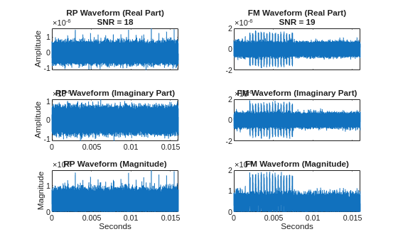
RPLFM simulated radar data set. The figure shows six signals in the time domain.

This data set comprises 900 simulated radar waveforms in noise designed to model realistic spectrum-sharing scenarios in the Citizens Broadband Radio Service (CBRS) band at 3.5 GHz [17]. The data is collected at a sample rate of 10 MHz for 80 milliseconds.

The data set contains two subfolders, comprising training data and test data.

  • The training data comprises 400 rectangular-pulse (RP) radar waveforms and 400 linear-frequency-modulated (LFM) radar waveforms.

  • The test data comprises 50 RP radar waveforms and 50 LFM radar waveforms.

  • All the waveforms have complex-valued white Gaussian noise added to achieve a realistic simulation environment.

To learn more about this data set, expand these sections.

Download the data set programmatically.

url = "https://www.mathworks.com/supportfiles/SPT/data/RPLFMSimulatedRadarDataset.zip";
downloadFolder = fullfile(tempdir,"RPLFMSimulatedRadarDataset");
zipFile = fullfile(downloadFolder,"RPLFMSimulatedRadarDataset.zip");
% Check if data set already exists. Otherwise, download it and unzip
if ~exist(fullfile(downloadFolder,"RPLFMSimulatedRadarDataset"),"dir")
    if ~exist(downloadFolder,"dir")
        mkdir(downloadFolder);
    end
    websave(zipFile,url);
    unzip(zipFile,downloadFolder);
end

Load the signal data.

% Define data set location
datasetLocation = fullfile(tempdir,"RPLFMSimulatedRadarDataset");
trainDataPath = fullfile(datasetLocation,"traindata");
testDataPath = fullfile(datasetLocation,"testdata");
% Load training labels and metadata
trainLabels = load(fullfile(trainDataPath,"RPFMradardataTrainLabels.mat"));
trainMetaData = load(fullfile(trainDataPath,"RPFMradardataTrainmetaData.mat"));
% Load test labels and metadata
testLabels = load(fullfile(testDataPath,"RPFMradardataTestLabels.mat"));
testMetaData = load(fullfile(testDataPath,"RPFMradardataTestmetaData.mat"));
% Display data set information
fprintf("Training samples: %d\n",length(trainLabels.RPFMradardataTrainLabels));
fprintf("Test samples: %d\n",length(testLabels.RPFMradardataTestLabels));
fprintf("\nTraining labels distribution:\n");
summary(trainLabels.RPFMradardataTrainLabels)

Read and preview one sample.

% Display waveform specifications
fprintf("Waveform specifications:\n");
fprintf("  Duration: %.4f seconds\n", ...
    trainMetaData.RPFMradardataTrainmetaData.duration(1));
fprintf("  Sample rate: %.0f Hz\n", ...
    trainMetaData.RPFMradardataTrainmetaData.SamplingFrequency(1));
fprintf("  Samples per waveform: %.0f\n", ...
    trainMetaData.RPFMradardataTrainmetaData.duration(1) * ...
    trainMetaData.RPFMradardataTrainmetaData.SamplingFrequency(1));
% Preview first 5 training samples metadata
fprintf("\nFirst 5 training samples:\n");
fprintf("  Sample 1: %s, PW=%.2e s, PRF=%d Hz, SNR=%d dB\n", ...
    string(trainMetaData.RPFMradardataTrainmetaData.BinNo(1)), ...
    trainMetaData.RPFMradardataTrainmetaData.PulseWidth(1), ...
    trainMetaData.RPFMradardataTrainmetaData.PulsesPerSecond(1), ...
    trainMetaData.RPFMradardataTrainmetaData.SNR(1));
fprintf("  Sample 2: %s, PW=%.2e s, PRF=%d Hz, SNR=%d dB\n", ...
    string(trainMetaData.RPFMradardataTrainmetaData.BinNo(2)), ...
    trainMetaData.RPFMradardataTrainmetaData.PulseWidth(2), ...
    trainMetaData.RPFMradardataTrainmetaData.PulsesPerSecond(2), ...
    trainMetaData.RPFMradardataTrainmetaData.SNR(2));
fprintf("  Sample 3: %s, PW=%.2e s, PRF=%d Hz, SNR=%d dB\n", ...
    string(trainMetaData.RPFMradardataTrainmetaData.BinNo(3)), ...
    trainMetaData.RPFMradardataTrainmetaData.PulseWidth(3), ...
    trainMetaData.RPFMradardataTrainmetaData.PulsesPerSecond(3), ...
    trainMetaData.RPFMradardataTrainmetaData.SNR(3));
% Show label distribution
fprintf("\nTest labels distribution:\n");
summary(testLabels.RPFMradardataTestLabels)

Structure:

RPLFMSimulatedRadarDataset/
├── license.txt
├── traindata/
│   ├── RPFMradardataTrain.mat         (1.83 GB - waveform data)
│   ├── RPFMradardataTrainLabels.mat   (780 bytes - categorical labels)
│   └── RPFMradardataTrainmetaData.mat (36 KB - 800×16 table)
└── testdata/
    ├── RPFMradardataTest.mat              (234.52 MB - waveform data)
    ├── RPFMradardataTestLabels.mat        (634 bytes - categorical labels)
    ├── RPFMradardataTestmetaData.mat      (6.3 KB - 100×16 table)
    └── trainedRadarDetectorMAP30.mat      (33 MB - pre-trained YOLOX model)

File details:

  • Size:

    • ZIP file: 2.1 GB

    • Extracted folder: 2.2 GB

    • Training data (RPFMradardataTrain.mat): 1.83 GB

    • Test data (RPFMradardataTest.mat): 234.52 MB

    • Pretrained data (trainedRadarDetectorMAP30.mat): 33 MB

  • Signals: 900 (800 for training, 100 for testing)

  • Labels: P0N#1 (RP waveform) or Q3N#3 (LFM waveform)

  • Metadata fields: 16 columns (BinNo, PulseWidth, PulsesPerSecond, PulsesPerBurst, ChirpWidth, ChirpDirection, SamplingFrequency, ActualPulseWidth, PhaseCodingType, SUID, radarStatus, radarSignalCenterFreq, radarSignalStartTime, SNR, NoisePowerdBmPerMHz, and duration)

Rectangular-pulse waveform specifications (each pulse has randomly set parameters):

  • Pulse width: from 0.5 to 2.5 microseconds

  • Pulse repetition frequency: from 900 to 1100 Hz

  • Number of pulses: from 15 to 40

  • Label: P0N#1

Linear-FM-pulse waveform specifications (each pulse has randomly set parameters):

  • Pulse width: from 50 to 100 microseconds

  • Pulse repetition frequency: from 300 to 3000 Hz

  • Chirp width: from 50 to 100 MHz

  • Chirp direction: up and down

  • Envelope: rectangular

  • Label: Q3N#3

Noise specifications:

  • Type: Complex-valued white Gaussian noise

  • SNR: from 17 to 20 dB (each waveform has a randomly set SNR)

Ultra-Wideband Radar Sensed Gestures

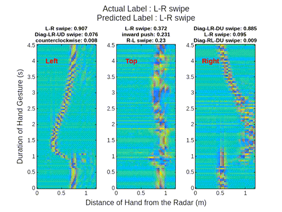
Ultra-wideband radar sensed Gestures data set. The figure shows eight signals in the time domain.

This data set comprises 9,600 radar-sensed 2-D recordings of 12 dynamic hand gestures [18], gathered from eight different human volunteers.

To obtain each recording, the examiners placed a separate UWB impulse radar at the left, top, and right sides of their experimental setup, resulting in three received radar signal data matrices.

  • The data set contains eight subfolders with 12 radar files. Each folder corresponds to a subject and each file corresponds to a hand gesture, for a total of 96 trials stored in 96 MAT files.

  • Each radar file has three matrices, each one corresponding to a radars used in the experimental setup: Left, Top, and Right.

  • Each matrix has 100 recordings concatenated from top to bottom and has a size of 9,000 × 189 (slow-time × fast-time bins). Each matrix is labeled as the hand gesture that generated it.

Movement-based signal data acquired using sensors, like UWB impulse radars, contain patterns specific to different gestures. Correlating motion data with movement benefits several avenues of work, including hand gesture recognition for contactless human-computer interaction.

To learn more about this data set, expand these sections.

Download the data set programmatically.

% Download and extract the UWB-gestures data set
dataUrl = "https://ssd.mathworks.com/supportfiles/SPT/data/uwb-gestures.zip";
downloadFolder = fullfile(tempdir,"UWBGestures");
zipFile = fullfile(downloadFolder,"uwb-gestures.zip");
% Check if data set already exists. Otherwise, download it and unzip
if ~exist(fullfile(downloadFolder,"uwb-gestures"),"dir")
    if ~exist(downloadFolder,"dir")
        mkdir(downloadFolder);
    end
    % Download data set
    websave(zipFile,dataUrl);
    unzip(zipFile,downloadFolder);
end

Load the signal data.

% Create signalDatastore to manage the radar data files
datasetLocation = fullfile(tempdir,"UWBGestures","uwb-gestures");
sds = signalDatastore(datasetLocation, ...
    IncludeSubfolders=true, ...
    SignalVariableNames=["Left" "Top" "Right"], ...
    FileExtensions=".mat", ...
    ReadOutputOrientation="row");
% Display data set information
fprintf("Total number of files: %d\n",numel(sds.Files));

Read and preview one sample.

% Read one sample from the datastore
[data,info] = read(sds);
% Display sample information
fprintf("Sample information:\n");
fprintf("  Filename: %s\n",info.FileName);
fprintf("  Number of radar channels: %d\n",length(data));
fprintf("  Left channel size: [%s]\n",num2str(size(data{1})));
fprintf("  Top channel size: [%s]\n",num2str(size(data{2})));
fprintf("  Right channel size: [%s]\n",num2str(size(data{3})));
fprintf("  Slow-time samples: %d\n",size(data{1},1));
fprintf("  Fast-time samples: %d\n",size(data{1},2));
% Reset datastore to the beginning
reset(sds);

Size:

  • ZIP file: 3.5 GB

  • Extracted folder: 3.5 GB

  • Signal data (each MAT file): ~36 MB

Structure:

uwb-gestures/
├── HV_01/
│   ├── HV_01_G01_RawData.mat (Left, Top, Right matrices 9000×189)
│   ├── HV_01_G02_RawData.mat
│   └── ... (12 gesture files)
├── HV_02/
│   └── ... (12 gesture files)
├── HV_03/
│   └── ... (12 gesture files)
├── HV_04/
│   └── ... (12 gesture files)
├── HV_05/
│   └── ... (12 gesture files)
├── HV_06/
│   └── ... (12 gesture files)
├── HV_07/
│   └── ... (12 gesture files)
└── HV_08/
    └── ... (12 gesture files)

File details:

  • Total files: 96 MAT files (8 volunteers × 12 gestures)

  • Variables per file: 3 (Left, Top, Right radar channels)

  • Matrix dimensions: 9,000 × 189 per channel

  • Gesture classes: 12 balanced classes

  • Samples per file: 100 gesture motions

  • Frames per gesture: 90 slow-time frames

  • Fast-time bins: 189 (spatial resolution)

  • Total samples: 9,600 (96 files × 100 samples/file)

Volunteers performed hand gestures from a gesture vocabulary consisting of 12 dynamic hand movements:

  1. Left-right swipe (L-R swipe)

  2. Right-left swipe (R-L swipe)

  3. Up-down swipe (U-D swipe)

  4. Down-up swipe (D-U swipe)

  5. Diagonal-left-right-up-down swipe (Diag-LR-UD swipe)

  6. Diagonal-left-right-down-up swipe (Diag-LR-DU swipe)

  7. Diagonal-right-left-up-down swipe (Diag-RL-UD swipe)

  8. Diagonal-right-left-down-up swipe (Diag-RL-DU swipe)

  9. Clockwise rotation

  10. Counterclockwise rotation

  11. Inward push

  12. Empty gesture

Continuous-Wave (CW) Radar Health Monitoring

Continuous-wave radar health monitoring data set. The figure shows eight signals in the time domain.

This data set comprises 2,060 files (1,030 CW radar segments and 1,030 ECG segments) of non-contact vital signs gathered from six healthy adult subjects [19]. The data is collected at a downsampled sample rate of 200 Hz for 5.12 seconds per segment.

The data set contains two subfolders, comprising training/validation data and test data.

  • The training/validation set is collected from subjects 1-5 and has 830 segments (704 for training and 126 for validation).

  • The test set is collected from subject 6 and has 200 segments.

The recordings were collected in controlled laboratory settings with subjects in seated or resting positions under normal respiration conditions.

  • The radar signals capture chest wall motion caused by cardiopulmonary activity, with frequency content primarily in the vital signs band (0.5-20 Hz), normalized to arbitrary units. These signals contain physiological information including heartbeat (mechanical cardiac contractions detected via chest displacement), respiration (breathing rate from thoracic expansion/contraction), heart rate variability (beat-to-beat interval variations), and respiratory sinus arrhythmia (heart rate modulation with breathing cycles).

  • The synchronized ECG reference signals are normalized by subtracting the median and rescaling so the maximum peak equals 1, providing ground-truth cardiac timing aligned with radar measurements.

The time-aligned radar and ECG data enable development of systems that map radar signals to cardiac metrics, supporting applications in remote patient monitoring, sleep apnea detection, elderly care, infant monitoring, smart home health monitoring, and vital signs monitoring in environments where contact sensors are impractical.

To learn more about this data set, expand these sections.

Download the data set programmatically.

% Download and extract the CW Radar Health Monitoring data set
dataUrl = "https://ssd.mathworks.com/supportfiles/SPT/data/SynchronizedRadarECGData.zip";
downloadFolder = fullfile(tempdir,"CWRadarHealth");
zipFile = fullfile(downloadFolder,"SynchronizedRadarECGData.zip");
% Check if data set already exists. Otherwise, download it and unzip
if ~exist(fullfile(downloadFolder,"trainVal"),"dir")
    if ~exist(downloadFolder,"dir")
        mkdir(downloadFolder);
    end
    % Download data set
    websave(zipFile,dataUrl);
    unzip(zipFile,downloadFolder);
end

Load the signal data.

% Create signalDatastore for radar and ECG data
trainFolder = fullfile(tempdir,"CWRadarHealth","trainVal");
testFolder = fullfile(tempdir,"CWRadarHealth","test");
% Training/validation datastore - radar signals
sds_radar_train = signalDatastore(fullfile(trainFolder,"radar"), ...
    IncludeSubfolders=true,FileExtensions=".mat");
% Training/validation datastore - ECG reference
sds_ecg_train = signalDatastore(fullfile(trainFolder,"ecg"), ...
    IncludeSubfolders=true,FileExtensions=".mat");
% Test datastore - radar signals
sds_radar_test = signalDatastore(fullfile(testFolder,"radar"), ...
    IncludeSubfolders=true,FileExtensions=".mat");
% Test datastore - ECG reference
sds_ecg_test = signalDatastore(fullfile(testFolder,"ecg"), ...
    IncludeSubfolders=true,FileExtensions=".mat");
% Display data set information
fprintf("Training/Validation radar files: %d\n",numel(sds_radar_train.Files));
fprintf("Training/Validation ECG files: %d\n",numel(sds_ecg_train.Files));
fprintf("Test radar files: %d\n",numel(sds_radar_test.Files));
fprintf("Test ECG files: %d\n",numel(sds_ecg_test.Files));

Read and preview one sample.

% Preview one synchronized radar and ECG pair
[radarData,radarInfo] = read(sds_radar_train);
reset(sds_radar_train);
[ecgData,ecgInfo] = read(sds_ecg_train);
reset(sds_ecg_train);
% Display radar signal information
fprintf("Radar Signal:\n");
fprintf("  Filename: %s\n",radarInfo.FileName);
fprintf("  Samples: %d\n",length(radarData));
fprintf("  Duration: %.2f seconds\n",length(radarData)/200);
fprintf("  Sample rate: 200 Hz\n");
fprintf("  Value range: [%.4f, %.4f]\n",min(radarData),max(radarData));
% Display ECG reference information
fprintf("\nECG Reference:\n");
fprintf("  Filename: %s\n",ecgInfo.FileName);
fprintf("  Samples: %d\n",length(ecgData));
fprintf("  Duration: %.2f seconds\n",length(ecgData)/200);
fprintf("  Sample rate: 200 Hz\n");
fprintf("  Value range: [%.4f, %.4f]\n",min(ecgData),max(ecgData));

Structure:

CWRadarHealth/
├── trainVal/                       (Training/Validation - 830 segments)
│   ├── ecg/                        (ECG reference signals)
│   │   ├── GDN0001_Resting_ecg_1.mat
│   │   ├── ...
│   │   ├── GDN0001_Valsalva_ecg_1.mat
│   │   ├── ...
│   │   ├── GDN0004_Apnea_ecg_1.mat
│   │   └── ... (830 files)
│   └── radar/                      (Radar signals)
│       ├── GDN0001_Resting_radar_1.mat
│       ├── ...
│       ├── GDN0001_Valsalva_radar_1.mat
│       ├── ...
│       ├── GDN0004_Apnea_radar_1.mat
│       └── ... (830 files)
├── test/                           (Test set - 200 segments)
│   ├── ecg/
│   │   ├── GDN0006_Resting_ecg_1.mat
│   │   ├── ...
│   │   ├── GDN0006_Valsalva_ecg_1.mat
│   │   ├── ...
│   │   ├── GDN0006_Apnea_ecg_1.mat
│   │   └── ... (200 files)
│   └── radar/
│       ├── GDN0006_Resting_radar_1.mat
│       ├── ...
│       ├── GDN0006_Valsalva_radar_1.mat
│       ├── ...
│       ├── GDN0006_Apnea_radar_1.mat
│       └── ... (200 files)
├── readme.txt
└── license.txt

File details:

  • Size:

    • ZIP file: 16 MB

    • Extracted folder: ~17 MB

    • Signal data (each MAT file): ~8-10 KB

  • Total files: 2,060 MAT files

    • Training/Validation: 1,660 files (830 radar + 830 ECG)

    • Test: 400 files (200 radar + 200 ECG)

  • Radar files:

    • Variables:radar_l (processed radar signal)

    • Size: 1-by-1024]

    • Sample rate: 200 Hz (downsampled)

    • Duration: ~5.12 seconds

    • Storage: Double-precision floating-point

    • Normalization: Arbitrary units

  • ECG files:

    • Variables:ecg_l (normalized ECG signal)

    • Size: 1-by-1024

    • Sample rate: 200 Hz (downsampled)

    • Duration: ~5.12 seconds

    • Normalization: Median-subtracted, max-peak scaled to 1

Data set statistics:

  • Total subjects: 6 healthy adults

  • Training subjects: 5 (subjects 1-5)

    • Training segments: 704

    • Validation segments: 126

  • Test subjects: 1 (subject 6, held-out)

    • Test segments: 200

  • Total segments: 1,030

  • Samples per segment: 1,024

  • Total radar samples: 1,054,720

  • Total ECG samples: 1,054,720

  • Total recording time: ~88 minutes (~1.5 hours)

Synchronization:

  • Radar and ECG recorded simultaneously

  • Time-aligned at 200 Hz

  • Matching filenames for paired signals (same subject/segment ID)

Radio-Frequency (RF) Frame Detection

RF frame detection data set. The figure shows eight signals in the time domain.

This data set comprises 4,831 complex I/Q baseband signals and a pretrained network [20]. The data is collected at a sample rate of 25 MHz for an average duration of 4.5 milliseconds.

The data set contains labeled radio frequency (RF) signal recordings from software-defined radio (SDR) captures of real-world wireless transmissions in the 2.4 GHz ISM band for identifying wireless communication protocols. The data set includes six RF signal classes:

  • BLE_1MHz — Bluetooth® Low Energy (BLE) 1 MHz bandwidth with frequency-hopping spread spectrum for IoT devices.

  • BLE_2MHz — Bluetooth Low Energy (BLE) 2 MHz bandwidth with extended advertising mode for high-throughput devices.

  • BT_classic — Bluetooth Classic BR/EDR with 1 MHz channels for audio streaming and phone calls.

  • WLAN — Wi-Fi® 802.11b/g/n with OFDM or DSSS modulation and 20-22 MHz channels for wireless networking.

  • Collision — Overlapping transmissions from multiple standards with superimposed frequency patterns.

  • Undefined — Background noise without active transmissions for idle spectrum detection.

You can obtain signal spectrograms using a 256-sample Hann window, 50% overlap between adjoining segments, 256 discrete Fourier transform points, producing time-frequency images with magnitude in dB scale and -80 dB minimum threshold. The high sample rate and detailed time-frequency domain representation enable effective spectrum sensing for cognitive radio and coexistence management in crowded RF environments.

To learn more about this data set, expand these sections.

Download the data set programmatically.

dataUrl = "https://ssd.mathworks.com/supportfiles/SPT/data/SpectrogramRFFrameDetectionData.zip";
downloadFolder = fullfile(tempdir,"RFFrameDetection");
zipFile = fullfile(downloadFolder,"SpectrogramRFFrameDetectionData.zip");
% Check if data set already exists. Otherwise, download it and unzip
if ~exist(fullfile(downloadFolder,"SpectrogramRFFrameDetectionData"),"dir")
    if ~exist(downloadFolder,"dir")
        mkdir(downloadFolder);
    end
    % Download data set
    websave(zipFile,dataUrl);
    unzip(zipFile,downloadFolder);
end

Load the signal data.

% Create signalDatastore for RF frame data
dataFolder = fullfile(tempdir,"RFFrameDetection","SpectrogramRFFrameDetectionData");
% Create datastore for all MAT files
sds = signalDatastore(dataFolder, ...
    IncludeSubfolders=true, ...
    FileExtensions=".mat");
% Display data set information
fprintf("RF Frame Detection Data set:\n");
fprintf("Total signal files: %d\n",numel(sds.Files));
% Preview one signal to check structure
[data,info] = read(sds);
reset(sds);
if iscell(data)
    signal = data{1};
else
    signal = data;
end
fprintf("\nSignal characteristics:\n");
fprintf("  Samples: %d\n",length(signal));
fprintf("  Duration: %.6f seconds\n",length(signal) / 25e6);
fprintf("  Data type: %s\n",class(signal));
fprintf("  Is complex: %s\n",string(~isreal(signal)));

Read and preview one sample.

% Load one RF frame sample
dataFolder = fullfile(tempdir,"RFFrameDetection","SpectrogramRFFrameDetectionData");
sds = signalDatastore(dataFolder,IncludeSubfolders=true,FileExtensions=".mat");
% Preview first signal
[data,info] = read(sds);
reset(sds);
% Extract signal
if iscell(data)
    signal = data{1};
else
    signal = data;
end
% Display sample information
fprintf("RF Signal Sample:\n");
fprintf("  Filename: %s\n",info.FileName);
fprintf("  Total samples: %d\n",length(signal));
fprintf("  Duration: %.6f seconds\n",length(signal) / 25e6);
fprintf("  Complex signal: %s\n",string(~isreal(signal)));
% Generate spectrogram for visualization/training
fs = 25e6;
[s,f,t] = stft(signal,fs,Window=hann(256),OverlapLength=128,FFTLength=256);
% Convert to dB and clip
dBSpec = mag2db(abs(s));
dBSpec(dBSpec < -80) = -80;
fprintf("\nSpectrogram dimensions:\n");
fprintf("  Frequency bins: %d\n",size(dBSpec,1));
fprintf("  Time frames: %d\n",size(dBSpec,2));
fprintf("  Power range: [%.1f, %.1f] dB\n",min(dBSpec(:)),max(dBSpec(:)));

Structure:

RFFrameDetection/
├── SpectrogramRFFrameDetectionData/        (4,832 RF signal MAT files)
│   ├── frame_138769090412766230_bw_25E+6.mat
│   ├── frame_138769090412766231_bw_25E+6.mat
│   ├── frame_138769090431506400_bw_25E+6.mat
│   └── ... (4,832 files total)
├── SpectrogramRFFrameDetectionNetwork/     (Pretrained networks)
│   └── networks.mat                         (301 MB)

Naming convention:

  • Format: frame_{timestamp}_bw_25E+6.mat

  • {timestamp}, unique identifier (Unix timestamp-based).

  • bw_25E+6 indicates 25 MHz bandwidth (25E+6 = 25×106 Hz).

Data structure in each MAT file:

  • Each file contains complex-valued samples in the I/Q (in-phase and quadrature) format.

  • Dimensions: 1-by-112,499 complex single, where N varies by signal segment duration.

File details:

  • Size:

    • ZIP file: 3.21 GB

    • Extracted folder: ~3.6 GB

    • Signal data (each MAT file): ~700 KB - 1 MB (variable size)

    • Pretrained network models (SpectrogramRFFrameDetectionNetwork/networks.mat file): 301 MB

  • Total files: 4,832 MAT files + 1 pretrained network

  • Signal classes: 6 categories (BLE_1MHz, BLE_2MHz, BT_classic, WLAN, Collision, or Undefined).

  • Samples per file: 112,499 samples (consistent across files)

  • Average duration: ~4.5 milliseconds per segment (4,500 µs)

  • Data type: Complex single-precision (I/Q)

  • Data properties:

    • Balanced classes: Equal representation of all 6 signal types

    • Real-world data: Captured from actual wireless devices

    • Augmented: Time shifts and SNR variations applied

    • Collision scenarios: Realistic overlapping transmissions

    • Noise included: Undefined class for idle spectrum

  • Class characteristics:

    Signal TypeBandwidthFrequency HoppingTypical DurationSpectral Signature
    BLE_1MHz1 MHzYes (37-40 channels)376 μs - 2 msNarrow band, hopping
    BLE_2MHz2 MHzYesVariableWider bandwidth
    BT_classic1 MHzYes (79 channels)625 μs slotsDense hopping
    WLAN20-22 MHzNoVariable burstsWide OFDM spectrum
    CollisionMixedMixedVariableOverlapped patterns
    UndefinedN/AN/ANoise onlyFlat spectrum

References

[1] Verma, N. K., Sevakula, R. K., Dixit, S., & Salour, A. (2016). "Intelligent Condition Based Monitoring Using Acoustic Signals for Air Compressors." IEEE Transactions on Reliability, Vol. 65, Number 1, pp. 291–309.

[2] Goldberger, A. L., Amaral, L. A. N., Glass, L., Hausdorff, J. M., Ivanov, P. Ch., Mark, R. G., Mietus, J. E.,, Moody, G. B. , Peng, C.-K., and Stanley, H. E. (2000) "PhysioBank, PhysioToolkit, and PhysioNet: Components of a New Research Resource for Complex Physiologic Signals". Circulation, Vol. 101, Number 23, pp. e215-e220.

[3] Liu et al. "An open access database for the evaluation of heart sound algorithms". (2016) Physiological Measurement, Vol. 37, Number 12, pp. 2181-2213.

[4] Giannoulis, D., Stowell, D., Benetos, E., Rossignol, M., Lagrange, M., and Plumbley, M. D. (2013) "A database and challenge for acoustic scene classification and event detection." 21st European Signal Processing Conference (EUSIPCO 2013), pp. 1–5.

[5] Stowell, D., Giannoulis, D., Benetos, E., Lagrange, M., and Plumbley, M. D. (2015) "Detection and Classification of Acoustic Scenes and Events." IEEE Transactions on Multimedia, Vol. 17, Number 10, pp. 1733–46.

[6] Jakobovski. “Jakobovski/Free-Spoken-Digit-Dataset.” GitHub, May 30, 2019. https://github.com/Jakobovski/free-spoken-digit-dataset.

[7] Mozilla Common Voice Corpus, https://commonvoice.mozilla.org/.

[8] Laguna, P., Mark, R. G., Goldberger, A. L., and Moody, G. B. (1997) "A Database for Evaluation of Algorithms for Measurement of QT and Other Waveform Intervals in the ECG." Computers in Cardiology, Vol. 24, pp. 673–676.

[9] Laguna, P., Jané, R., and Caminal, P. (1994) "Automatic detection of wave boundaries in multilead ECG signals: Validation with the CSE database." Computers and Biomedical Research, Vol. 27, Number 1, pp. 45–60.

[10] Chan, A. D. C., and Green, G. C. (2007) "Myoelectric Control Development Toolbox." 30th Conference of the Canadian Medical & Biological Engineering Society, Toronto, Canada.

[11] Moody, G. B., and Mark, R. G. (2001) "The impact of the MIT-BIH Arrhythmia Database." IEEE Engineering in Medicine and Biology Magazine, Vol. 20, Number 3, pp. 45–50.

[12] Moody, G. B., Muldrow, W. E., and Mark, R. G. (1984) "A noise stress test for arrhythmia detectors." Computers in Cardiology, Vol. 11, pp. 381–384.

[13] Andreotti, F., Behar, J., and Clifford, G. D. (2016) "Fetal ECG Synthetic Database" https://physionet.org/content/fecgsyndb/1.0.0/.

[14] Zhang, H., Zhao, M., Wei, C., Mantini, D., Li, Z., and Liu, Q. (2021) "EEGdenoiseNet: A Benchmark Dataset for End-to-End Deep Learning Solutions of EEG Denoising." arXiv:2009.11662 https://arxiv.org/abs/2009.11662.

[15] Andrzejak, R. G., Lehnertz, K., Mormann, F., Rieke, C., David, P., and Elger, C. E. (2001) "Indications of Nonlinear Deterministic and Finite-Dimensional Structures in Time Series of Brain Electrical Activity: Dependence on Recording Region and Brain State." Physical Review, Vol. 64, Number 6, pp. 61907–61914, https://doi.org/10.1103/physreve.64.061907.

[16] Mousavi, S. M., Sheng, Y. , Zhu, W., and Beroza, G. C. (2019) "STanford EArthquake Dataset (STEAD): A Global Data Set of Seismic Signals for AI." IEEE Access, Vol. 7, pp. 179464–76.

[17] Caromi, R., Souryal, M., and Hall, T. A. (2017). "RF Dataset of Incumbent Radar Signals in the 3.5GHz CBRS Band." Journal of Research of the National Institute of Standards and Technology, Vol. 124, Number 124038.

[18] Ahmed, S., Wang, D., Park, J., et al. (2021). "UWB-gestures, a public dataset of dynamic hand gestures acquired using impulse radar sensors." Scientific Data, Vol. 8, Article 102.

[19] Schellenberger, S., Shi, K., Steigleder, T. et al. (2020) "A dataset of clinically recorded radar vital signs with synchronized reference sensor signals." Scientific Data, Vol. 7, Article 291.

[20] Wicht, J., Wetzker, U., and Jain, V. (2022). Spectrogram Data Set for Deep Learning Based RF-Frame Detection. Data, Vol. 7, Number 12, p. 168.

See Also

Topics