freqzmr

Compute DTFT approximation of impulse response of multirate or single-rate filter

Since R2024a

Syntax

[Y,Fout] = freqzmr(filtObj)

freqzmr(filtObj)

Description

[Y,Fout] = freqzmr(filtObj) outputs the impulse response discrete-time Fourier transform (DTFT) and corresponding frequencies of the filter object specified in filtObj.

If the input filter is a single-rate FIR or IIR filter, the behavior of freqzmr and freqz functions is equivalent. If the filter is an irreducible multirate filter, use the freqzmr function to analyze the frequency response of the filter. For more details on the differences between these two functions, see Comparison of freqzmr and freqz functions. For more information on reducible and irreducible multirate filters, see Overview of Multirate Filters.

example

freqzmr(filtObj) plots the magnitude and phase of the impulse response DTFT. The function also color-codes the distortion caused by the rate changes. For more information on distortion, see Output Distortion.

example

Examples

collapse all

Impulse Response DTFT of FIR Rate Converter

Open Live Script

Compute and plot the impulse response DTFT of FIR rate converter using the freqzmr function.

firRC = dsp.FIRRateConverter(5,7);
freqzmr(firRC)

Figure Output spectrum (one sided) contains 2 axes objects. Axes object 1 with title Output Magnitude, xlabel Frequency (mHz), ylabel Magnitude (dB) contains an object of type patch. Axes object 2 with title Output Phase, xlabel Frequency (mHz), ylabel Phase (rad) contains an object of type line.

Impulse Response DTFT of Sample Rate Converter

Open Live Script

Compute the impulse response DTFT of sample rate converter using the freqzmr function.

SRC = dsp.SampleRateConverter(InputSampleRate=77,...
                               OutputSampleRate=32*24,...
                               Bandwidth=23,...
                               StopbandAttenuation=120);
 
[Y,F] = freqzmr(SRC,MinimumFFTLength=1024);

When you do not specify any output arguments, the function plots the impulse response DTFT on a convenience plot.

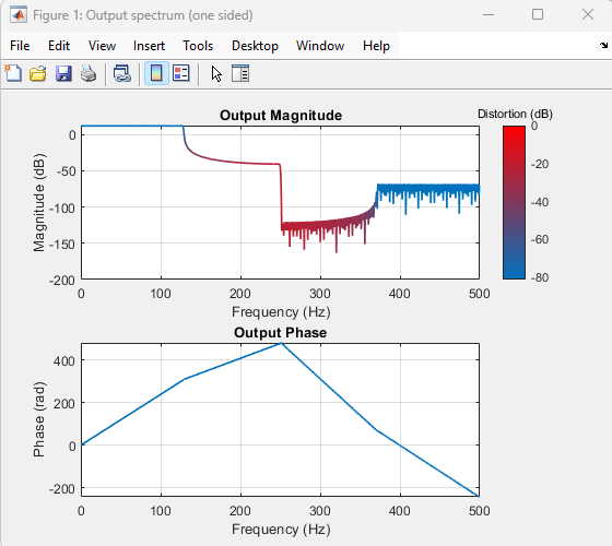
Plot the impulse response DTFT with maximum distortion sensitivity. In the red regions in the plot, you can expect some distortion due to the rate-conversion aliasing.

freqzmr(SRC,MinimumFFTLength=1024,DistortionThreshold=-inf);

Figure Output spectrum (one sided) contains 2 axes objects. Axes object 1 with title Output Magnitude, xlabel Frequency (Hz), ylabel Magnitude (dB) contains an object of type patch. Axes object 2 with title Output Phase, xlabel Frequency (Hz), ylabel Phase (rad) contains an object of type line.

To hide distortion coloring, set DistortionThreshold to 0.

freqzmr(SRC,MinimumFFTLength=1024,DistortionThreshold=0);

Figure Output spectrum (one sided) contains 2 axes objects. Axes object 1 with title Output Magnitude, xlabel Frequency (Hz), ylabel Magnitude (dB) contains an object of type line. Axes object 2 with title Output Phase, xlabel Frequency (Hz), ylabel Phase (rad) contains an object of type line.

Specify the frequency range to be "centered".

freqzmr(SRC,MinimumFFTLength=1024,DistortionThreshold=-inf,FrequencyRange="centered");

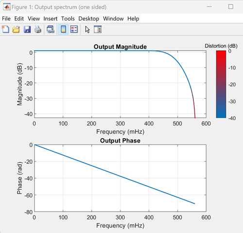
Figure Output spectrum contains 2 axes objects. Axes object 1 with title Output Magnitude, xlabel Frequency (Hz), ylabel Magnitude (dB) contains an object of type patch. Axes object 2 with title Output Phase, xlabel Frequency (Hz), ylabel Phase (rad) contains an object of type line.

To compare, pass a random white noise signal to the sample rate converter. View the spectrum of the corresponding output in the spectrum analyzer.

You can see that the impulse response DTFT that freqzmr function computes is exactly the same as the spectrum of the output signal when you input a random white noise signal.

sa = spectrumAnalyzer(SampleRate=SRC.OutputSampleRate,PlotAsTwoSidedSpectrum=true,YLimits=[-200 20]);

for k=1:10
    u = randn(4096,1);
    y = SRC(u);
    sa(y);
end

Impulse Response DTFT of Composite Filter

Open Live Script

Design a composite filter that is a cascade of these filters:

Single-rate filter
Parallel structure of multirate filters

Design the single-rate filter using the dsp.LowpassFilter object in its default configuration.

singleRateFilter = dsp.LowpassFilter

singleRateFilter = 
  dsp.LowpassFilter with properties:

               FilterType: 'FIR'
    DesignForMinimumOrder: true
        PassbandFrequency: 8000
        StopbandFrequency: 12000
           PassbandRipple: 0.1000
      StopbandAttenuation: 80
      NormalizedFrequency: false
               SampleRate: 44100

  Use get to show all properties

The parallel structure contains a cascade of dsp.FIRInterpolator and dsp.FIRDecimator objects and a dsp.FIRRateConverter object.

Design the dsp.FIRInterpolator and the dsp.FIRRateConverter objects using the designBandpassFIR function.

B1 = 2.5*designBandpassFIR(FilterOrder=256,...
    CenterFrequency=0.3,Bandwidth=1/5);
B2 = 0.25*designBandpassFIR(FilterOrder=256,...
    CenterFrequency=0.7,Bandwidth=1/20);

Create a parallel structure of multirate filters using the parallel and cascade functions.

multirateFilter = parallel(cascade(dsp.FIRInterpolator(5,B1),...
    dsp.FIRDecimator(2)),dsp.FIRRateConverter(10,4,B2))

multirateFilter = 
  dsp.ParallelFilter with properties:

          Branch1: [1x1 dsp.FilterCascade]
          Branch2: [1x1 dsp.FIRRateConverter]
    CloneBranches: true

Create a composite filter that is a cascade of the single-rate filter and the parallel filter.

compositeFilter = cascade(singleRateFilter,multirateFilter)

compositeFilter = 
  dsp.FilterCascade with properties:

         Stage1: [1x1 dsp.LowpassFilter]
         Stage2: [1x1 dsp.ParallelFilter]
    CloneStages: true

Compute and plot the impulse response DTFT of this filter using the freqzmr function. Set MinimumFFTLength to 512. Set the frequency range to be "centered".

freqzmr(compositeFilter,MinimumFFTLength=512,FrequencyRange='centered')

Figure Output spectrum contains 2 axes objects. Axes object 1 with title Output Magnitude, xlabel Frequency (kHz), ylabel Magnitude (dB) contains an object of type patch. Axes object 2 with title Output Phase, xlabel Frequency (kHz), ylabel Phase (rad) contains an object of type line.

Input Arguments

collapse all

Name-Value Arguments

Specify optional pairs of arguments as Name1=Value1,...,NameN=ValueN, where Name is the argument name and Value is the corresponding value. Name-value arguments must appear after other arguments, but the order of the pairs does not matter.

Example: src = dsp.SampleRateConverter(InputSampleRate=77,OutputSampleRate=32*24,Bandwidth=23,StopbandAttenuation=120); [Y,Fout] = freqzmr(src,MinimumFFTLength=1024,DistortionThreshold=-inf);

`MinimumFFTLength` — Shortest discrete spectrum length
512 (default) | positive integer

Shortest discrete spectrum length, specified as a positive integer. When the function resamples the spectrum internally (for example, during downsampling), the size of the resampled spectrum is no shorter than MinimumFFTLength. For more information, see DTFT of Downsampled Signal.

Data Types: double

`InputSampleRate` — Sample rate of input signal in Hz
positive integer

Sample rate of the input signal FsIn in Hz, specified as a positive integer.

If you do not specify the input sample rate, the function inherits this value from the filter object. If the input filter object contains an explicit property to specify the input sample rate, the function uses the value of that property. If the filter object does not contain any such property, the function uses a value of 1.

Data Types: double

`FrequencyRange` — Frequency range of DTFT
`"auto"` (default) | `"onesided""twosided"` | `"centered"`

Frequency range of the DTFT, specified as one of these:

"auto" –– The function automatically determines the appropriate choice ("onesided" or "twosided") based on the system symmetry. The function selects "onesided" when the system spectrum is Hermitian symmetric and "twosided" otherwise.
"onesided" –– Impulse response DTFT contains only the positive frequencies. Frequency range is [0 F_sout/2].
"twosided" –– Frequency range is [0 F_sout].
"centered" –– Frequency range is [−F_sout/2 F_sout/2].

F_sout is the output sample rate and is given by the equation F_sout = F_sIn×(L/M), where L/M is the rate conversion ratio of the input filter object.

`DistortionThreshold` — Distortion threshold to determine ambiguity
`-40` (default) | scalar in the range (−∞ 0]

Distortion threshold in dB to determine ambiguity in the convenience magnitude plot, specified as a scalar in the range (−∞ 0]. The DistortionThreshold argument is the threshold over which the signal is considered ambiguous.

Decrease the threshold value for a more sensitive detection of distortion. The function colors the convenience magnitude plot according to the distortion ratio. Red indicates maximum distortion (two or more branches have the same power), while blue indicates no distortion. If the distortion threshold is 0 dB, the function hides all distortion coloring.

The function ignores any distortion value below the value of DistortionThreshold and treats the output as non-ambiguous.

Here is a plot of the impulse response DTFT of an FIR rate converter with the distortion threshold of −∞. This plot shows the most sensitive detection of distortion.

Magnitude plot shows bright distinction between the red and blue areas in the distortion.

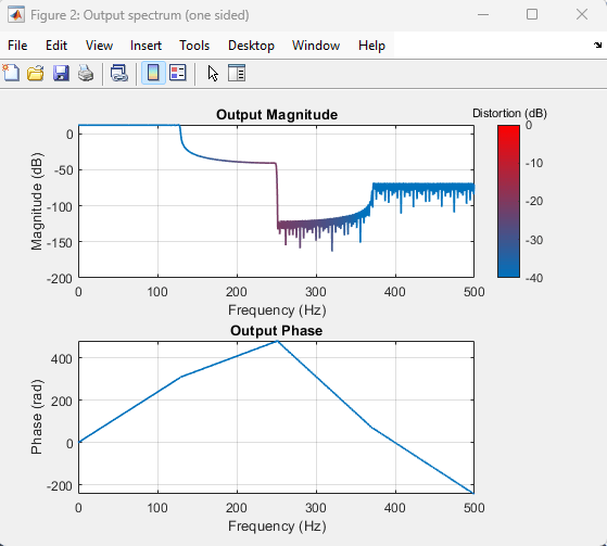
Increase the threshold value to −40 dB. The function ignores all distortions below −40 dB.

Magnitude plot shows bright distinction between the red and blue areas in the distortion.

Increasing the threshold value to 0 dB shows no distortion on the plot because the function ignores all the distortion values.

Magnitude plot shows no distortion.

For more information, see Output Distortion.

Data Types: double

Output Arguments

collapse all

`Y` — DTFT approximation of impulse response
column vector

DTFT approximation of the impulse response, returned as a column vector. The length of the impulse response DTFT depends on the MinimumFFTLength value and the rate conversion factors of the multirate filter stages.

Data Types: double
Complex Number Support: Yes

`Fout` — Output frequencies in Hz
column vector

Output frequencies in Hz corresponding to the impulse response DTFT approximation, returned as a column vector. The length of Fout equals the length of Y. The range of Fout depends on the FrequencyRange.

Data Types: double

More About

collapse all

Discrete-Time Fourier Transform (DTFT) and DFT and FFT

The discrete-time Fourier transform (DTFT) of a sequence x[m] sampled at rate T is a periodic complex-valued function and is given by

$X_{1 / T} (f) = {\sum_{m} x [m] e}^{- 2 π j f \cdot T \cdot m}$

, where T is the sample rate of the signal. DTFT plays a central role in the analysis of discrete signals and systems.

For computational purposes, DTFT is sampled on a finite set of frequencies and can be expressed in terms of DFT and FFT.

Comparison of `freqzmr` and `freqz` functions

The freqz function plots the frequency response of a single-rate FIR or IIR filter, while the freqzmr function plots the DTFT approximation of the filter impulse response. This distinction stems from the fact that multirate filters, in general, do not have a frequency response because a single input tone can generate multiple output tones. The freqzmr function accounts for multirate operations in its DTFT approximation, while freqz assumes that the filter is a single-rate FIR or IIR filter.

Here are a few examples which illustrate the behavior of freqz and freqzmr for single-rate filters and various types of multirate filters.

Single-Rate Filters

For single-rate FIR or IIR filters, the frequency response is equal to the DTFT of their impulse response, and the behavior of freqzmr and freqz functions is equivalent.

Consider the dsp.LowpassFilter object which is a single-rate filter.

lpFilter = dsp.LowpassFilter

Plot the frequency response of this filter using freqz and the DTFT of the impulse response using freqzmr. Overlay the two plots.

The two plots are exactly the same.

Multirate Filters

Multirate filters cannot be characterized by a single transfer function and do not have a frequency response in the usual sense. However, multirate filters have a well-defined impulse response, whose DTFT gives valuable information about the spectral content of their outputs.

The freqzmr function computes the DTFT approximation of the multirate filter impulse response and accounts for multirate operations while doing so. This behavior allows the freqzmr function to capture multirate effects such as imaging and aliasing, while the freqz function does not capture those effects.

This filter is an antialiasing FIR filter with a downsample factor of 4.

firDec = dsp.FIRDecimator(4)

The freqz function inspects this filter as a single-rate filter. The freqzmr function computes the DTFT approximation of the filter impulse response. The DTFT plot accounts for aliasing and looks different compared to the frequency response plot. The aliased components compensate to a flat response. The plot shows these components by coloring them in red. For more information, see Output Distortion.

Multirate filters can be reducible or irreducible. A multirate filter is said to be reducible if it can be modified through noble identities to produce a single-rate FIR or IIR filter, as firDec in the previous example. For more information, see Overview of Multirate Filters. If the input filter is a reducible multirate filter, you can use the freqz function to analyze the filter. The function analyzes the equivalent FIR or IIR stage and treats the filter as a single-rate FIR or IIR filter.

Multirate Filter Reducing to a Single-Stage Filter

Consider this FIR rate converter which is trivially reducible for it has a single FIR stage.

firrc = dsp.FIRRateConverter(3,2,triang(9))

firrc = 
  dsp.FIRRateConverter with properties:

   Main
    InterpolationFactor: 3
       DecimationFactor: 2
        NumeratorSource: 'Property'
              Numerator: [9×1 double]

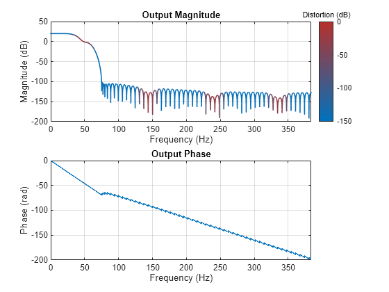
With an input sample rate of 1 kHz, the output sample rate is 1.5 kHz. Plot the frequency response of the filter using freqz, and the DTFT of the filter impulse response using freqzmr. You can see that there is distortion in the frequency range [0.4 0.75 kHz]. The DTFT plot shows this distortion.

Consider this filter that is a cascade of a lowpass filter and an FIR rate converter. You can reduce this filter to a single stage.

lpfilt = dsp.LowpassFilter(SampleRate=1e3,...
PassbandFrequency=80,StopbandFrequency=100,FilterType='IIR');
firrc = dsp.FIRRateConverter(3,4);
cascFilt = cascade(lpfilt,firrc)

cascFilt = 

  dsp.FilterCascade with properties:

         Stage1: [1×1 dsp.LowpassFilter]
         Stage2: [1×1 dsp.FIRRateConverter]
    CloneStages: true

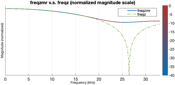
Plot the frequency response of this filter using freqz and the DTFT of the filter impulse response using freqzmr. Overlay and compare the two plots.

The two functions generate plots that look similar but are not the same. The freqzmr plot shows the distortion regions in red, where there is rate-conversion aliasing.

Irreducible Multirate Filter

Lastly, if the input filter is an irreducible multirate filter, use the freqzmr function to analyze the filter in the frequency domain. For more information on irreducible filters, see Overview of Multirate Filters.

Consider this filter that is a cascade of two FIR rate converters. This filter is irreducible.

firrc1 = dsp.FIRRateConverter;
firrc2 = dsp.FIRRateConverter(3,4);
cascFilt = cascade(firrc1,firrc2)

cascFilt = 

  dsp.FilterCascade with properties:

         Stage1: [1×1 dsp.FIRRateConverter]
         Stage2: [1×1 dsp.FIRRateConverter]
    CloneStages: true

When you try to analyze this filter with freqz, the function errors out.

To analyze this filter, use the freqzmr function, which in its default configuration shows the DTFT of the filter impulse response.

freqzmr(src)

To summarize, for irreducible multirate filters, use the freqzmr function. For single-rate FIR or IIR filters, the behavior of freqz and freqzmr is equivalent.

Here is a table that compares the two functions and lists the key differences.

	`freqzmr`	`freqz`
Computation	DTFT approximation of filter impulse response h DTFT(h)	Frequency response of the filter, which is the transfer function evaluated on the unit circle
Single-rate convolution filters	✓	✓
Reducible multirate filters	✓	✓ Performs analysis on the single-rate FIR or IIR equivalent. The plot looks different compared to the `freqzmr` plot.
Irreducible multirate filters	✓	╳
Captures multirate effects such as imaging an aliasing	✓	╳
Support for normalized frequencies	╳	✓

Algorithms

collapse all

The freqzmr algorithm treats the input filter object as a combination of FIR or IIR (single-rate) filters and multirate operations (upsample and downsample). The function processes the DTFT through each stage consecutively. For more information on DTFT, see Discrete-Time Fourier Transform (DTFT) and DFT and FFT.

Single-Rate FIR or IIR Filters

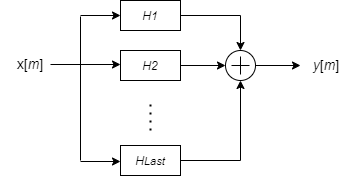
Here is the block diagram of a single-rate filter with an input sequence x[m] and an output sequence y[m].

where h is the impulse response of the single-rate filter.

The freqzmr function computes the impulse response DTFT, that is, DTFT(h).

DTFT of Downsampled Signal

For a given input signal x[m], the output of the downsampling operation is given by y[n] = x[Mm].

The DTFT of the downsampled signal is periodic and its period 1/(MT) is 1/M of the period of X_1/T.

$Y_{1 / (M T)} (f) = \frac{1}{M} \sum_{m = 0}^{M - 1} X_{1 / T} (\frac{f - m / T}{M})$

For multirate filters, the components in $X_{1 / T} (\frac{f - m / T}{M})$ can overlap and interfere with each other resulting in aliasing. To resolve aliasing, it is important that one of the components dominates the rest in its value. This component contributes to the sum while the rest are 0 and resolves the issue of aliasing. In most cases, this component corresponds to m=0 (baseband component), that is, Y_(1/MT)(f)≅X_1/T(f/M).

Multirate distortion is the level of ambiguity between these components. You can specify the threshold in dB over which the function considers the signal ambiguous using the DistortionThreshold property. For more information, see Output Distortion.

Computing the DTFT of Downsampled Signal

DTFT downsampling is done through reshaping of the DTFT samples vector and taking a sum across columns. To downsample a signal with DTFT samples vector X by a decimation factor M, the downsampled DTFT is:

NX = size(X,1);
Y = (1/M)*sum(reshape(X,NX/M,M),2);

The DTFT array X is usually resampled at a higher frequency resolution (increase by NX) prior to reshaping. This is done in order to make the NX length divisible by M and to ensure that the resolution of the downsampled DTFT Y is no less than MinimumFFTLength.

DTFT of Upsampled Signal

For a given input signal x[m], the output of the upsampling operation is given by

$y [n] = {\begin{matrix} x [k] & m = k L \\ 0 & e l s e \end{matrix}$

y[n] operates at a rate L/T. The DTFT of the upsampled signal y is identical to the DTFT of x, that is, Y_L/T(f) = X_1/T(f). The only difference is in the period, which is L/T, that is, L times larger on the frequency domain.

The freqzmr function determines the DTFT of the upsampled signal by replicating the input DTFT samples vector L times.

function Y = upsampleDTFT(X,L)    
    Y = repmat(X,L,1);
end

DTFT of Composite Filters (Cascade and Parallel)

Cascade Filters

For a cascade of filters, the freqzmr function computes the output DTFT by passing the output DTFT of each stage as the input DTFT of the following stage. The first stage input is an impulse.

freqzmr(cascade(H1,H2)) = freqzmr(H2,...
InputSpectrum=freqzmr(H1))

If you have multiple stages in the cascade, the freqzmr function computes the impulse response DTFT using this logic.

function Y = cascadeDTFT(obj,X,MinimumFFTLength)
    Y = X;
    for k = 1:NumStages
       Y = outputDTFT(Stage(k),Y,MinimumFFTLength);
    end
end

Parallel Filters

For parallel filters, the DTFT output is a sum of the DTFTs of the filter outputs on the individual branches.

Output Distortion

In multirate systems, an input frequency generates several output frequencies due to aliasing and imaging. As a result, an output frequency component is often a combination of several different frequency components.

You can express the output DTFT of a multirate filter as a sum of the components Q₀, Q₁, …., Q_M-1.

$Y (f) = \sum_{m = 0}^{M - 1} Q_{m} (f)$

where:

M is the total decimation factor.
Q₀, Q₁, …., Q_M-1 are DTFT components that the function computes through rate change operations.

Ideally, only one branch contributes to the sum while the rest are 0 (no aliasing), that is, Q_m = 0 for all m except for one. As soon as more than one of the branches has a nonzero value, Y(f) exhibits aliasing.

The distortion is the level of ambiguity of the frequency branches Q_m(f) in the sum above. It is defined as the inverse power ratio between the dominant component and the average power of the remaining components.

$D (f) = \sqrt{\frac{Q_{m 1}}{(M - 1) \sum_{k = 2}^{M} {| Q_{m k} (f) |}^{2}}}$

The distortion ratio ranges between 0 and 1 (or −∞ to 0 in dB), where higher values indicate more ambiguity. A 1:1 ratio (0 dB) indicates that there is no dominant component, and the signal is totally ambiguous. In contrast, a 0-ratio (−∞ dB) indicates that the output frequency is non-ambiguous.

The freqzmr function sorts m₁, …., m_M at every frequency according to the corresponding Q_m magnitude values. The distortion ratio is invariant under permutations, that is, changing the order of the branches does not alter the distortion. The distortion ratio is a real number between 0 and 1. These values indicate where aliasing is present in a multirate system.

The function colors the impulse response DTFT depending on the value of the distortion ratio. Red indicates maximum distortion (two or more branches have the same power), while blue indicates no distortion. The function ignores any distortion value below the value specified in DistortionThreshold.

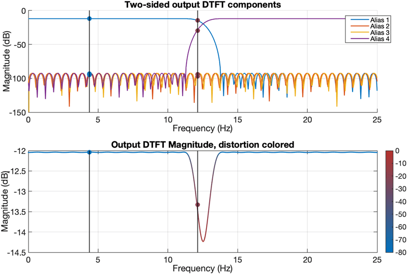
The following figure shows the distortion ratio in two frequencies. In the lower frequency (f = 4.375 Hz), there is a fairly low distortion since the dominant lobe is about 80 dB above the rest of the lobes. In the higher frequency (f = 12.125 Hz), there is far more significant interference as alias lobe 4 is much closer to the dominant lobe 1. This is indicated by the red color on the freqzmr plot.

Version History

Introduced in R2024a

expand all

R2024b: Support for `dsp.VariableFIRDecimator` and `dsp.VariableFIRInterpolator` Objects

Starting in R2024b, the freqzmr analysis function supports the dsp.VariableFIRDecimator and dsp.VariableFIRInterpolator objects.

R2024b: Support for `dsp.DCBlocker` object

Starting in R2024b, this function supports the dsp.DCBlocker object.

freqzmr

Syntax

Description

Examples

Impulse Response DTFT of FIR Rate Converter

Impulse Response DTFT of Sample Rate Converter

Impulse Response DTFT of Composite Filter

Input Arguments

`filtObj` — Input filter
filter System object™

Name-Value Arguments

`MinimumFFTLength` — Shortest discrete spectrum length
512 (default) | positive integer

`InputSampleRate` — Sample rate of input signal in Hz
positive integer

`FrequencyRange` — Frequency range of DTFT
`"auto"` (default) | `"onesided""twosided"` | `"centered"`

`DistortionThreshold` — Distortion threshold to determine ambiguity
`-40` (default) | scalar in the range (−∞ 0]

Output Arguments

`Y` — DTFT approximation of impulse response
column vector

`Fout` — Output frequencies in Hz
column vector

More About

Discrete-Time Fourier Transform (DTFT) and DFT and FFT

Comparison of `freqzmr` and `freqz` functions

Algorithms

Single-Rate FIR or IIR Filters

DTFT of Downsampled Signal

DTFT of Upsampled Signal

DTFT of Composite Filters (Cascade and Parallel)

Output Distortion

Version History

R2024b: Support for `dsp.VariableFIRDecimator` and `dsp.VariableFIRInterpolator` Objects

R2024b: Support for `dsp.DCBlocker` object

See Also

Topics

freqzmr

Syntax

Description

Examples

Impulse Response DTFT of FIR Rate Converter

Impulse Response DTFT of Sample Rate Converter

Impulse Response DTFT of Composite Filter

Input Arguments

filtObj — Input filter filter System object™

Name-Value Arguments

MinimumFFTLength — Shortest discrete spectrum length 512 (default) | positive integer

InputSampleRate — Sample rate of input signal in Hz positive integer

FrequencyRange — Frequency range of DTFT "auto" (default) | "onesided""twosided" | "centered"

DistortionThreshold — Distortion threshold to determine ambiguity -40 (default) | scalar in the range (−∞ 0]

Output Arguments

Y — DTFT approximation of impulse response column vector

Fout — Output frequencies in Hz column vector

More About

Discrete-Time Fourier Transform (DTFT) and DFT and FFT

Comparison of freqzmr and freqz functions

Algorithms

Single-Rate FIR or IIR Filters

DTFT of Downsampled Signal

DTFT of Upsampled Signal

DTFT of Composite Filters (Cascade and Parallel)

Output Distortion

Version History

R2024b: Support for dsp.VariableFIRDecimator and dsp.VariableFIRInterpolator Objects

R2024b: Support for dsp.DCBlocker object

See Also

Topics

`filtObj` — Input filter
filter System object™

`MinimumFFTLength` — Shortest discrete spectrum length
512 (default) | positive integer

`InputSampleRate` — Sample rate of input signal in Hz
positive integer

`FrequencyRange` — Frequency range of DTFT
`"auto"` (default) | `"onesided""twosided"` | `"centered"`

`DistortionThreshold` — Distortion threshold to determine ambiguity
`-40` (default) | scalar in the range (−∞ 0]

`Y` — DTFT approximation of impulse response
column vector

`Fout` — Output frequencies in Hz
column vector

Comparison of `freqzmr` and `freqz` functions

R2024b: Support for `dsp.VariableFIRDecimator` and `dsp.VariableFIRInterpolator` Objects

R2024b: Support for `dsp.DCBlocker` object