Diversify ESG Portfolios

Open Live Script

This example shows how to include qualitative factors for environmental, social, and corporate governance (ESG) in the portfolio selection process. The example extends the traditional mean-variance portfolio using a Portfolio object to include the ESG metric. First, the estimateFrontier function computes the mean-variance efficient frontier for different ESG levels. Then, the example illustrates how to combine the ESG performance measure with portfolio diversification techniques. Specifically, it introduces hybrid models that use the Herfindahl-Hirshman (HH) index and the most diversified portfolio (MDP) approach using the estimateCustomObjectivePortfolio function. Finally, the backtestEngine framework compares the returns and behavior of the different ESG strategies.

Define Mean-Variance Portfolio

Load the table with the asset returns and a vector with ESG scores for the assets. Both the asset returns and their ESG scores are simulated values and do not represent the performance of any real securities. However, you can apply the code and workflow in this example to any data set with prices and returns and ESG information.

% Load data
load('asset_return_100_simulated.mat') % Returns table
load('ESG_s26.mat')                    % ESG scores

Transform the returns table into a prices timetable.

% Transform returns to prices
assetPrices = ret2tick(stockReturns);
% Transform prices table to timetable
nRows = size(stockReturns,1);
day = datetime("today");
Time = (day-nRows):day;
assetPrices = table2timetable(assetPrices,"RowTimes",Time);

Define a Portfolio object with default constraints where the weights must be nonnegative and sum to 1.

% Create a mean-variance Portfolio object with default constraints
p = Portfolio;
p = estimateAssetMoments(p,stockReturns);
p = setDefaultConstraints(p);

Compute the Mean-Variance Efficient Frontier for Different ESG Levels

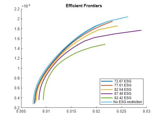
Obtain contour plots of the ESG-mean-variance efficient surface. You obtain the efficient surface from the Pareto optima of the multiobjective problem that includes all the performance metrics: average ESG score, average return, and return variance.

First, obtain feasible values of the ESG metric by finding the minimum and maximum ESG levels. To do this step, use the estimateCustomObjectivePortfolio function assigning the average ESG score as the objective function. The average ESG score of a portfolio is the weighted sum of the individual asset ESG scores, where the weights are given by the amount invested in each asset.

% Define objective function: average ESG score
ESGscore = @(x) ESGnumeric'*x;

% Find the minimum ESG score
solMin = estimateCustomObjectivePortfolio(p,ESGscore);
minESG = ESGscore(solMin)

minESG = 
0.0187

% Find the maximum ESG score
solMax = estimateCustomObjectivePortfolio(p,ESGscore, ...
    ObjectiveSense="maximize");
maxESG = ESGscore(solMax)

maxESG = 
0.9735

To compute the contours of the efficient surface, you add the average ESG score as a constraint using the setInequality function. The coefficients of the linear constraint are the ESG scores associated with each asset and the right-hand side is the target ESG score for the desired contour. Notice that the convention of the inequalities in the Portfolio object is $\leq$ . Because the goal is to maximize the average ESG score, the target ESG value for the contour should be a lower bound. Therefore, you need to flip the signs of the coefficients and the right-hand side of the added inequality. The function that computes and plots the contours is in the Local Functions section.

N = 20; % Number of efficient portfolios per ESG value

% Add ESG score as a constraint to the Portfolio object
Ain = -ESGnumeric';
bin = -minESG; % Start with the smallest ESG score
p = setInequality(p,Ain,bin);

% Esimate lower value for contour plots
pwgt = estimateFrontier(p,N);
pESG = pwgt'*ESGnumeric;
minContour = max(pESG); % All ESG scores lower than this have
                        % overlapped contours.

% Plot contours
nC = 5; % Number of contour plots
plotESGContours(p,ESGnumeric,minContour,maxESG,nC,N);

Figure contains an axes object. The axes object with title Efficient Frontiers contains 6 objects of type line. These objects represent 72.67 ESG, 77.61 ESG, 82.54 ESG, 87.48 ESG, 92.42 ESG, No ESG restriction.

Diversification Techniques

In this example, the two diversification measures are the equally weighted (EW) portfolio and the most diversified portfolio (MDP).

You obtain the EW portfolio using the Herfindahl-Hirschman (HH) index as the diversification measure

$HH (x) = \sum_{i = 1}^{n} x_{i}^{2}$

An equally weighted portfolio minimizes this index. Therefore, the portfolios that you obtain from using this index as a penalty have weights that satisfy the portfolio constraints and are more evenly weighted.

The diversification measure for the most diversified portfolio (MDP) is

$MDP (x) = - \sum_{i = 1}^{n} σ_{i} x_{i}$

where $σ_{i}$ represents the standard deviation of asset $i$ . Using this measure as a penalty function maximizes the diversification ratio [1].

$φ (x) = \frac{x^{T} σ}{\sqrt{x^{T} Σ x}}$

If the portfolio is fully invested in one asset, or if all assets are perfectly correlated, the diversification ratio $φ (x)$ is equal to 1. For all other cases, $φ (x) > 1$ . Therefore, if $φ (x) \approx 1$ , there is no diversification, so the goal is to maximize $φ (x)$ . Unlike the HH index, the goal of MDP is not to obtain a portfolio whose weights are evenly distributed among all assets, but to obtain a portfolio whose selected (nonzero) assets have the same correlation to the portfolio as a whole.

Diversification for Fixed ESG Level

You can extend the traditional minimum variance portfolio problem subject to an expected return to include the ESG metric by setting an ESG constraint for the problem. The purpose of the ESG constraint is to force the portfolio to achieve an ESG score greater than a certain target. Then, add a penalty term to the objective function to guide the problem toward more or less diversified portfolios. How diversified a portfolio is depends on your choice of the penalty parameter.

Choose an ESG level of 0.85 and an expected return of 0.001.

% Minimum ESG and return levels
ESG0 = 0.85;
ret0 = 1e-3;

Currently, the portfolio problem assumes that the weights must be nonnegative and sum to 1. Add the requirement that the return of the portfolio is at least ret0 and the ESG score is at least ESG0. The feasible set is represented as $X$ , which is

$X = {x | x \geq 0, \sum_{i = 1}^{n} x_{i} = 1, μ^{T} x \geq {ret}_{0}, ESG (x) \geq {ESG}_{0}}$

Add the ESG constraint using the setInequality function.

% Add ESG constraint
Ain = -ESGnumeric';
bin = -ESG0; % Set target ESG score
p = setInequality(p,Ain,bin);

To add the return constraint, pass the name-value argument TargetReturn=ret0 to the estimateCustomObjectivePortfolio function for each of the different custom objective portfolios of interest.

The portfolio that minimizes the variance with the HH penalty is

$\min_{x \in X} x^{T} Σ x + λ_{HH} x^{T} x$

% HH penalty parameter
lambdaHH =0.001;
% Variance + Herfindahl-Hirschman (HH) index
var_HH = @(x) x'*p.AssetCovar*x + lambdaHH*(x'*x);
% Solution that accounts for risk and HH diversification
wHHMix = estimateCustomObjectivePortfolio(p,var_HH,TargetReturn=ret0);

The portfolio that minimizes the variance with the MDP penalty is

$\min_{x \in X} x^{T} Σ x - λ_{MDP} σ^{T} x$

% MDP penalty parameter
lambdaMDP =0.01;
% Variance + Most Diversified Portfolio (MDP)
sigma = sqrt(diag(p.AssetCovar));
var_MDP = @(x) x'*p.AssetCovar*x - lambdaMDP*(sigma'*x);
% Solution that accounts for risk and MDP diversification
wMDPMix = estimateCustomObjectivePortfolio(p,var_MDP,TargetReturn=ret0);

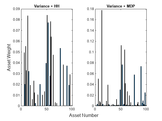
Plot the asset allocation from the penalized strategies.

% Plot asset allocation
figure
t = tiledlayout(1,2);

% HH penalized method
nexttile    
bar(wHHMix');
title('Variance + HH')

% MDP penalized method
nexttile
bar(wMDPMix')
title('Variance + MDP')

% General labels
ylabel(t,'Asset Weight')
xlabel(t,'Asset Number')

Figure contains 2 axes objects. Axes object 1 with title Variance + HH contains an object of type bar. Axes object 2 with title Variance + MDP contains an object of type bar.

The strategies that include the penalty function in the objective give weights that are between the minimum variance portfolio weights and the weights from the respective maximum diversification technique. In fact, for the problem with the HH penalty, choosing $λ_{HH} = 0$ returns the minimum variance solution, and as $λ_{HH} \to \infty$ , the solution approaches the one that maximizes HH diversification. For the problem with the MDP penalty, choosing $λ_{MDP} = 0$ also returns the minimum variance solution, and there exists a value ${\hat{λ}}_{MDP}$ such that the MDP problem and the penalized version are equivalent. Consequently, values of $λ_{MDP} \in [0, {\hat{λ}}_{MDP}]$ return asset weights that range from the minimum variance behavior to the MDP behavior.

Diversification by "Tilting"

The strategies in Diversification for Fixed ESG Level explicitly set a target ESG average score. However, a different set of strategies controls the ESG score in a less direct way. The method in these strategies uses ESG tilting. With tilting, you discretize the ESG score into 'high' and 'low' levels and the objective function penalizes each level differently. In other words, you use the diversification measure to tilt the portfolio toward higher or lower ESG values. Therefore, instead of explicitly requiring that the portfolios maintain a target ESG average score, you select assets, with respect to their ESG score, implicitly through the choice of penalty parameters.

Start by labeling the assets with an ESG score less than or equal to 0.5 as 'low' and assets with an ESG score greater than 0.5 as 'high', and then remove the ESG constraint.

% Label ESG data
ESGlabel = discretize(ESGnumeric,[0 0.5 1], ...
    "categorical",{'low','high'});
% Create table with ESG scores and labels
ESG = table(ESGnumeric,ESGlabel);
% Remove ESG constraint
p = setInequality(p,[],[]);

The tilted version of the portfolio with the HH index is

$\begin{array}{l} \min x^{T} Σ x + λ_{HH}^{high} \sum_{i \in H} x_{i}^{2} + λ_{HH}^{low} \sum_{i \in L} x_{i}^{2} \\ s . t . \sum_{i = 1}^{n} x_{i} = 1, μ^{T} x \geq {ret}_{0}, x \geq 0 \end{array}$

The feasible region does not bound the average ESG level of the portfolio. Instead, you implicitly control the ESG score by applying different penalization terms to assets with a 'high' ESG score ( $i \in H$ ) and assets with a 'low' ESG score ( $i \in L$ ). To achieve a portfolio with a high average ESG score, the penalty terms must satisfy that $0 \leq λ_{HH}^{high} \leq λ_{HH}^{low}$ .

% HH penalty parameters
% Penalty parameter for assets with 'low' ESG score
lambdaLowHH =0.01;
% Penalty parameter for assets with 'high' ESG score
lambdaHighHH =0.001;
% Lambda for HH 'tilted' penalty
lambdaTiltHH = (ESG.ESGlabel=='low').*lambdaLowHH + (ESG.ESGlabel=='high').*lambdaHighHH;

% Variance + Herfindahl-Hirschman (HH) index
tilt_HH = @(x) x'*p.AssetCovar*x + lambdaTiltHH'*(x.^2);
% Solution that minimizes variance + HH term
wTiltHH = estimateCustomObjectivePortfolio(p,tilt_HH,TargetReturn=ret0);

Similarly, the tilted version of the portfolio with the MDP penalty term is given by

$\begin{array}{l} \min x^{T} Σ x - λ_{MDP}^{high} \sum_{i \in H} σ_{i} x_{i} - λ_{MDP}^{low} \sum_{i \in L} σ_{i} x_{i} \\ s . t . \sum_{i = 1}^{n} x_{i} = 1, μ^{T} x \geq {ret}_{0}, x \geq 0 \end{array}$

In this case, to achieve a portfolio with a high average ESG score, the penalty terms must satisfy that $0 \leq λ_{MDP}^{low} \leq λ_{MDP}^{high}$ .

% MDP penalty parameters
% Penalty parameter for assets with 'low' ESG score
lambdaLowMDP =0.001;
% Penalty parameter for assets with 'high' ESG score
lambdaHighMDP =0.01;
% Lambda for MDP 'tilted' penalty
lambdaTiltMDP = (ESG.ESGlabel=='low').*lambdaLowMDP + (ESG.ESGlabel=='high').*lambdaHighMDP;

% Variance + MDP index
tilt_MDP = @(x) x'*p.AssetCovar*x - lambdaTiltMDP'*(sigma.*x);
% Solution that minimizes variance + HH term
wTiltMDP = estimateCustomObjectivePortfolio(p,tilt_MDP,TargetReturn=ret0);

Compare ESG Scores

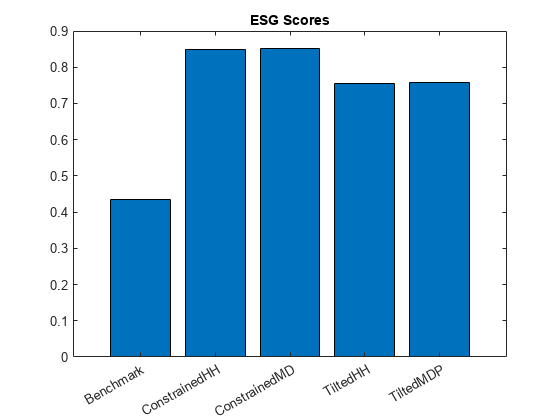
Compare the ESG scores using tilting and a target ESG constraint. For the comparison to be more meaningful, compute the minimum variance portfolio without ESG constraints or penalty terms, and use the ESG score of the minimum variance portfolio as benchmark.

% Compute the minimum variance portfolio without ESG constraints
p = setInequality(p,[],[]);
wBmk = estimateFrontierByReturn(p,ret0);

% Compute ESG scores for the different strategies
Benchmark = ESGnumeric'*wBmk;
ConstrainedHH = ESGnumeric'*wHHMix;
ConstrainedMD = ESGnumeric'*wMDPMix;
TiltedHH = ESGnumeric'*wTiltHH;
TiltedMDP = ESGnumeric'*wTiltMDP;

% Create table
strategiesESG = table(Benchmark,ConstrainedHH,ConstrainedMD,TiltedHH,TiltedMDP);
figure;
bar(categorical(strategiesESG.Properties.VariableNames),strategiesESG.Variables)
title('ESG Scores')

Figure contains an axes object. The axes object with title ESG Scores contains an object of type bar.

As expected, the ESG scores of the penalized strategies are better than the ESG scores of the minimum variance portfolio without constraint and penalty terms. However, the tilted strategies achieve lower ESG scores than the ones that include the target ESG score as a constraint. This comparison shows the flexibility of the tilted strategy. If the ESG target score is not an essential requirement, then you can consider a tilting strategy.

Backtest Using Strategies

To show the performance through time for the two strategies (Diversification for Fixed ESG Level and Diversification by "Tilting"), use the backtestEngine framework. Use backtestStrategy to compare the strategies with a prespecified target ESG score with the strategies that use ESG tilting.

% Store info to pass to ESG constrained strategies
Ain = -ESGnumeric';
bin = -ESG0; % Set target ESG score
conStruct.p = setInequality(p,-ESGnumeric',-ESG0);
conStruct.ret0 = ret0;
conStruct.lambdaHH =0.01;
conStruct.lambdaMDP =0.05;

% Store info to pass to ESG tilting strategies
tiltStruct.p = setInequality(p,[],[]);
tiltStruct.ret0 = ret0;
% HH tilting penalty parameters
% Penalty parameter for assets with 'low' ESG score
HHlambdaLow =0.1;
% Penalty parameter for assets with 'high' ESG score
HHlambdaHigh =0.01;
% Combined penalty terms for HH
tiltStruct.lambdaHH = (ESG.ESGlabel=='low').*HHlambdaLow + ...
    (ESG.ESGlabel=='high').*HHlambdaHigh;
% MDP tilting penalty parameters
% Penalty parameter for assets with 'low' ESG score
MDPlambdaLow =0.005;
% Penalty parameter for assets with 'high' ESG score
MDPlambdaHigh =0.05;
% Combined penalty terms for MDP
tiltStruct.lambdaMDP = (ESG.ESGlabel=='low').*MDPlambdaLow + ...
    (ESG.ESGlabel=='high').*MDPlambdaHigh;

Define the investment strategies that you want to use to make the asset allocation decisions at each investment period. For this example, four investment strategies are defined as input to backtestStrategy. The first two strategies require a minimum ESG score and the last two use the ESG tilting method.

% Define backtesting parameters
warmupPeriod = 84;       % Warmup period
rebalFreq = 42;          % Rebalance frequency
lookback  = [42 126];     % Lookback window
transactionCost = 0.001; % Transaction cost for trade
% Constrained variance + HH strategy
strat1 = backtestStrategy('MixedHH', @(w,P) MixHH(w,P,conStruct), ...
    'RebalanceFrequency', rebalFreq, ...
    'LookbackWindow', lookback, ...
    'TransactionCosts', transactionCost, ...
    'InitialWeights', wHHMix);
% Constrained variance + MDP
strat2 = backtestStrategy('MixedMDP', @(w,P) MixMDP(w,P,conStruct), ...
    'RebalanceFrequency', rebalFreq, ...
    'LookbackWindow', lookback, ...
    'TransactionCosts', transactionCost, ...
    'InitialWeights', wMDPMix);
% HH tilted strategy
strat3 = backtestStrategy('TiltedHH', @(w,P) tiltedHH(w,P,tiltStruct), ...
    'RebalanceFrequency', rebalFreq, ...
    'LookbackWindow', lookback, ...
    'TransactionCosts', transactionCost, ...
    'InitialWeights', wTiltHH);
% MDP tilted strategy
strat4 = backtestStrategy('TiltedMDP', @(w,P) tiltedMDP(w,P,tiltStruct), ...
    'RebalanceFrequency', rebalFreq, ...
    'LookbackWindow', lookback, ...
    'TransactionCosts', transactionCost, ...
    'InitialWeights', wTiltMDP);
% All strategies
strategies = [strat1,strat2,strat3,strat4];

Run the backtest using runBacktest and generate a summary for each strategy's performance results.

% Create the backtesting engine object
backtester = backtestEngine(strategies);
% Run backtest
backtester = runBacktest(backtester,assetPrices,...
    'Start',warmupPeriod);

% Summary
summary(backtester)

ans=9×4 table
                        MixedHH       MixedMDP      TiltedHH     TiltedMDP 
                       __________    __________    __________    __________

    TotalReturn            0.7077        1.1927       0.79527        1.3295
    SharpeRatio          0.029317       0.03188      0.031911      0.034608
    Volatility           0.011965      0.017845      0.011719      0.016851
    AverageTurnover     0.0054528     0.0065605     0.0053991     0.0070898
    MaxTurnover           0.80059       0.72624       0.80099       0.76676
    AverageReturn      0.00035068    0.00056875    0.00037387    0.00058304
    MaxDrawdown           0.23083       0.34334       0.22526       0.34688
    AverageBuyCost       0.068778      0.097277      0.070048       0.12019
    AverageSellCost      0.068778      0.097277      0.070048       0.12019

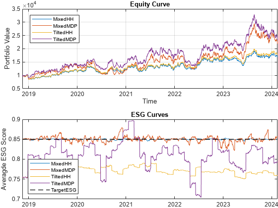
To visualize their performance over the entire investment period, plot the daily results of the strategies using equityCurve.

% Plot daily stocks and ESG strategy behavior
figure
t = tiledlayout(2,1,'Padding','none');

% Equity curves
nexttile(t)
equityCurve(backtester);

% Table and plot of the average ESG score for the mixed and tilted
% strategies throughout the investment period
nexttile(t)
TAvgESG = averageESGTimetable(backtester,ESGnumeric,ESG0);

Figure contains 2 axes objects. Axes object 1 with title Equity Curve, xlabel Time, ylabel Portfolio Value contains 4 objects of type line. These objects represent MixedHH, MixedMDP, TiltedHH, TiltedMDP. Axes object 2 with title ESG Curves, ylabel Averagde ESG Score contains 5 objects of type line. These objects represent MixedHH, MixedMDP, TiltedHH, TiltedMDP, TargetESG.

In the Equity Curve plot, the tilted MDP strategy is the one that performs the best by the end of the investment period, followed by the mixed MDP strategy with the ESG constraint. The performance of the mixed and tilted strategies depend on the choice of the penalty parameters. Both ESG methods, the constrained and the tilted methods, require defining two parameters for each strategy. The ESG constrained method requires you to provide a target ESG score and a penalty parameter for the diversification term. The ESG tilting requires one penalty parameter value for the assets with 'high' ESG scores and a different one for 'low' ESG scores. In addition, the ESG tilting requires a third parameter to determine the cutoff point between 'high' and 'low' ESG assets. Given the dependency of the penalized strategies on the value of their parameters, the performance of those strategies vary widely. However, this example shows that it is possible to find values of the parameters so that the resulting strategies obtain good returns while improving on the average ESG score.

The ESG Curves plot shows the average ESG evolution computed throughout the investment period for the penalized investment strategies, both for the ESG constrained method and the ESG tilting method. You can see that, unlike the choice of the ESG target for the ESG constraint, the selection of the tilting penalty parameters has an effect on the ESG score of the optimal portfolios that is less explicit. Therefore, the average ESG score varies more with the tilting strategies than with the constrained strategies, as expected.

Although not shown in this example, the traditional minimum variance portfolio strategy, subject to the same expected return and ESG levels, results in higher average turnover and transaction costs than any of the strategies covered in the example. Another advantage of adding a diversification measure to the formulation of the problem is to reduce the average turnover and transaction costs.

References

[1] Richard, J. C., and T. Roncalli. Smart Beta: Managing Diversification of Minimum Variance Portfolios. Risk-Based and Factor Investing. Elsevier, pp. 31-63, 2015.

Local Functions

function [] = plotESGContours(p,ESGscores,minESG,maxESG,nCont,...
    nPort)
% Plot mean-variance frontier for different ESG levels

% Add ESG constraint
p.AInequality = -ESGscores';

% Compute mean-variance risks and returns for different ESG levels
contourESG = linspace(minESG,maxESG,nCont+1);
figure
hold on
labels = strings(nCont+1,1);
for i = 1:nCont
    p.bInequality = -contourESG(i); % Change target ESG score
    plotFrontier(p,nPort);
    labels(i) = sprintf("%6.2f ESG",contourESG(i)*100);
end

% Plot the original mean-variance frontier
p.AInequality = []; p.bInequality = [];
plotFrontier(p,nPort);
labels(i+1) = "No ESG restriction";
title('Efficient Frontiers')
legend(labels,'Location','southeast')
hold off

end

function [ESGTimetable] = averageESGTimetable(backtester,...
    ESGscores,targetESG)
% Create a table of the average ESG score for the mix and tilted
% strategies throughout the investment period and plot it

% Normalize weights
wMixedHH = backtester.Positions.MixedHH{:,2:end}./...
    sum(backtester.Positions.MixedHH.Variables,2);
wMixedMDP = backtester.Positions.MixedMDP{:,2:end}./...
    sum(backtester.Positions.MixedMDP.Variables,2);
wTiltedHH = backtester.Positions.TiltedHH{:,2:end}./...
    sum(backtester.Positions.TiltedHH.Variables,2);
wTiltedMDP = backtester.Positions.TiltedMDP{:,2:end}./...
    sum(backtester.Positions.TiltedMDP.Variables,2);

% Compute ESG scores for the different strategies
consHH_ESG = wMixedHH*ESGscores;
consMDP_ESG = wMixedMDP*ESGscores;
tiltedHH_ESG = wTiltedHH*ESGscores;
tiltedMDP_ESG = wTiltedMDP*ESGscores;

% Create timetable
ESGTimetable = timetable(backtester.Positions.TiltedHH.Time,...
    consHH_ESG,consMDP_ESG,tiltedHH_ESG,tiltedMDP_ESG);

% Plot ESG curves
plot(ESGTimetable.Time, ESGTimetable.Variables);
hold on
plot(ESGTimetable.Time, targetESG*ones(size(ESGTimetable.Time)),...
    'k--','LineWidth',1); % Plots target ESG scores
title('ESG Curves');
ylabel('Averagde ESG Score');
legend('MixedHH','MixedMDP','TiltedHH','TiltedMDP', 'TargetESG',...
    'Location','southwest');

end

function new_weights = MixHH(~, assetPrices, struct)
% Min variance + max HH diversification strategy

% Retrieve portfolio information
p = struct.p;
ret0 = struct.ret0;

% Define returns and covariance matrix
assetReturns = tick2ret(assetPrices);
p = estimateAssetMoments(p,assetReturns{:,:});

% Objective function: Variance + Herfindahl-Hirschman
% diversification term
%   min x'*Sigma*x + lambda*x'*x
objFun = @(x) x'*p.AssetCovar*x + struct.lambdaHH*(x'*x);

% Solve problem
% Solution that minimizes the variance + HH index
new_weights = estimateCustomObjectivePortfolio(p,objFun,...
    TargetReturn=ret0);

end

function new_weights = MixMDP(~, assetPrices, struct)
% Min variance + MDP diversification strategy

% Retrieve portfolio information
p = struct.p;
ret0 = struct.ret0;

% Define returns and covariance matrix
assetReturns = tick2ret(assetPrices);
p = estimateAssetMoments(p,assetReturns{:,:});
sigma = sqrt(diag(p.AssetCovar));

% Objective function: Variance + MDP diversification term
%   min x'*Sigma*x - lambda*sigma'*x
objFun = @(x) x'*p.AssetCovar*x - struct.lambdaMDP*(sigma'*x);

% Solve problem
% Solution that minimizes variance + MDP term
new_weights = estimateCustomObjectivePortfolio(p,objFun,...
    TargetReturn=ret0);

end

function new_weights = tiltedHH(~,assetPrices,struct)
% Tilted HH approach

% Retrieve portfolio information
p = struct.p;
ret0 = struct.ret0;
lambda = struct.lambdaHH;

% Define returns and covariance matrix
assetReturns = tick2ret(assetPrices);
p = estimateAssetMoments(p,assetReturns{:,:});

% Objective function: Variance + Herfindahl-Hirschman
% diversification term
%   min x'*Sigma*x + lambda*x'*x
objFun = @(x) x'*p.AssetCovar*x + lambda'*(x.^2);

% Solve problem
% Solution that minimizes variance + HH term
new_weights = estimateCustomObjectivePortfolio(p,objFun,...
    TargetReturn=ret0);

end

function new_weights = tiltedMDP(~,assetPrices,struct)
% Tilted MDP approach

% Retrieve portfolio information
p = struct.p;
ret0 = struct.ret0;
lambda = struct.lambdaMDP;

% Define returns and covariance matrix
assetReturns = tick2ret(assetPrices);
p = estimateAssetMoments(p,assetReturns{:,:});
sigma = sqrt(diag(p.AssetCovar));

% Objective function: Variance + MDP
%   min x'*Sigma*x - lambda*sigma'*x
objFun = @(x) x'*p.AssetCovar*x - lambda'*(sigma.*x);

% Solve problem
% Solution that minimizes variance + MDP term
new_weights = estimateCustomObjectivePortfolio(p,objFun,...
    TargetReturn=ret0);

end

% The API of the rebalance functions (MixHH, MixMDP, tiltedHH, and
% tiltedMDP) require a first input with the current weights. They
% are redundant for these strategies and can be ignored.