Using Signal Analyzer App
App Workflow
A typical workflow for inspecting and comparing signals using the Signal Analyzer app is:
Select Signals to Analyze — Select any signal available in the MATLAB® workspace. The app accepts numeric arrays and signals with inherent time information, such as MATLAB
timetablearrays,timeseriesobjects, andlabeledSignalSetobjects. For more information, see Data Types Supported by Signal Analyzer. Add time information to signals using sample rates, numeric vectors,durationarrays, or MATLAB expressions.Preprocess Signals — Edit signals using trim, clip, split, extract, or crop actions. Lowpass, highpass, bandpass, or bandstop filter signals. Remove trends and compute signal envelopes. Smooth signals using moving averages, regression, Savitzky-Golay filters, or other methods. Denoise signals using wavelets. Find and fill missing data using moving average, autoregressive model, or other methods (since R2024a). Change sample rates of signals or interpolate nonuniformly sampled signals onto uniform grids. Preprocess signals using your own custom functions. Generate MATLAB functions to automate preprocessing operations.
Explore Signals — Play audio signals (since R2024a). Plot and compare data, their spectra, their spectrograms, or their scalograms. Look for features and patterns in the time domain, in the frequency domain, and in the time-frequency domain. Control leakage, resolution bandwidth, or window length when computing power spectra. Compute persistence spectra to analyze sporadic signals and sharpen spectrogram estimates using reassignment. Extract regions of interest from signals.
Measure Signals — Interactively measure signal, spectrum, and time-frequency data. Calculate time-domain signal statistics such as minimum, maximum, mean, and root-mean-square. Find and annotate signal peaks in the time domain. View statistics and peak values in a measurements table.
Share Analysis — Copy displays from the app to the clipboard as images. Export signals to the MATLAB workspace or save them to MAT-files. Generate MATLAB scripts to automate the computation of power spectrum, spectrogram, or persistence spectrum estimates and the extraction of regions of interest. Save Signal Analyzer sessions to resume your analysis later or on another machine.
Example: Extract Regions of Interest from Whale Song
Read an audio file that contains data from a Pacific blue whale, sampled at 4 kHz. The file is from the library of animal vocalizations maintained by the Cornell University Bioacoustics Research Program. The time scale in the data is compressed by a factor of 10 to raise the pitch and make the calls more audible. Convert the signal to a MATLAB® timetable.
[w,fs] = audioread("bluewhalesong.au");

whale = timetable(seconds((0:length(w)-1)'/fs),w);
Open Signal Analyzer and drag the timetable to a display. To hear audio signals, click Play in the Playback section of the toolstrip to play the entire signal once. Select Play in Loop and then click Play to play the signal repeatedly. Four features stand out from the noise. The first is known as a trill, and the other three are known as moans.

On the Display tab, click Spectrum to open a spectrum view and click Panner to activate the panner. Use the panner to create a zoom window with a width of about 2 seconds. Drag the zoom window so that it is centered on the trill. The spectrum shows a noticeable peak at around 900 Hz.

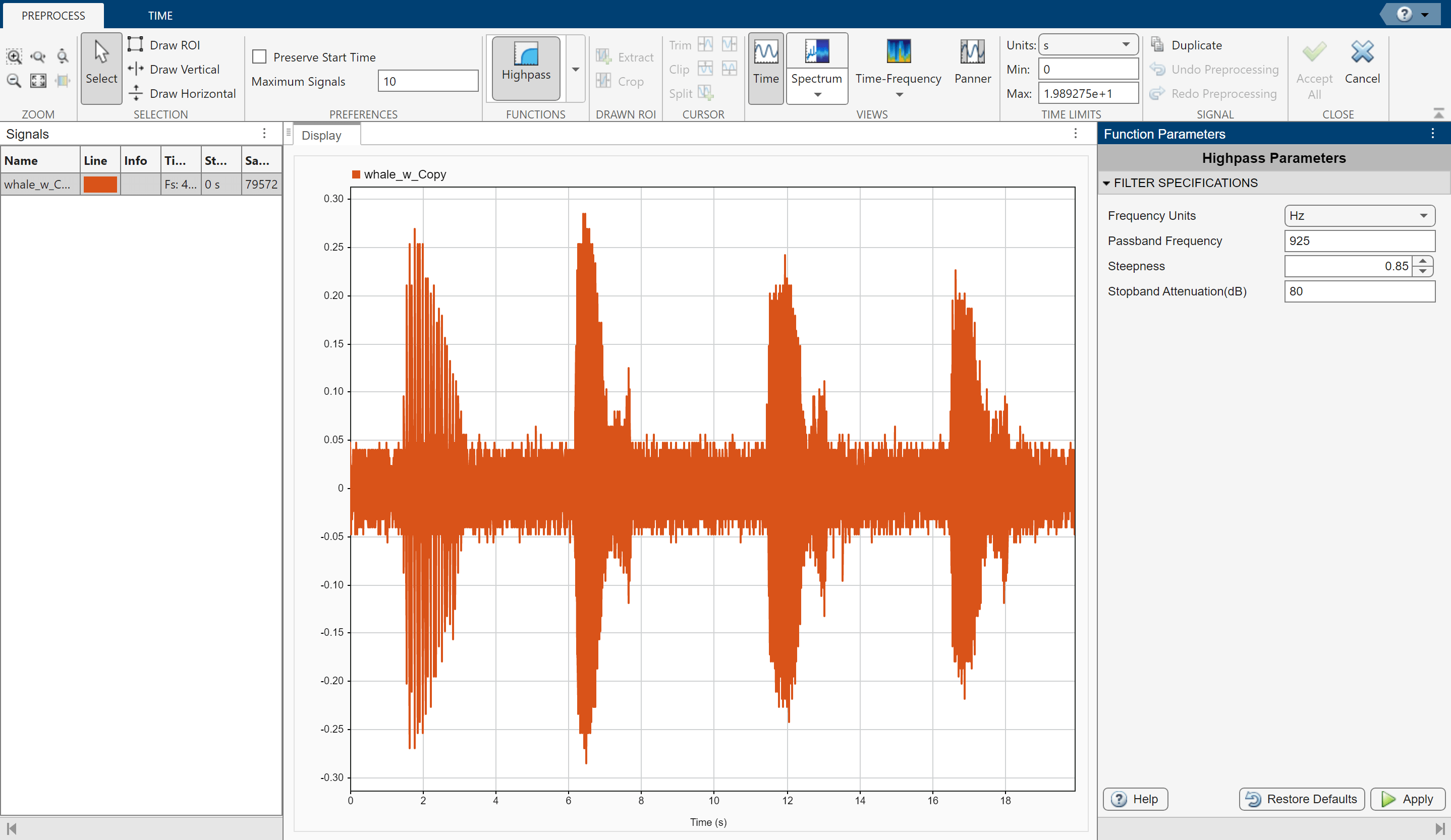
Isolate the single trill by highpass filtering. Right-click the signal in the Signal table and select Duplicate to create a copy of the whale song. Remove the original signal from the display by clearing the check box next to its name in the Signal table.
With the duplicate signal selected in the Signal table, on the Analyzer tab, click Preprocess. Select Highpass from the Functions gallery. In the Function Parameters panel, set the passband frequency to 925 Hz and the stopband attenuation to 80 dB. Use the default value for the steepness. Click Apply.
Go to the Display tab and place two data cursors by clicking the arrow below Data Cursors and selecting Two. Place one cursor at 1.3 second and the other cursor at 3.3 seconds. Click the arrow next to Extract Signals and select Between Time Cursors to extract the region containing the trill.

Clear the display and select the original signal. Extract the three moans to compare their spectra:
Center the panner zoom window on the first moan. The spectrum has eight clearly defined peaks, located very close to multiples of 170 Hz. Click the button next to Extract Signals and select
Between Time Limits.Click Panner to hide the panner. Press the space bar to see the full signal. Click Zoom in X and zoom in on a 2-second interval of the time view centered on the second moan. The spectrum again has peaks at multiples of 170 Hz. Click the button next to Extract Signals and select
Between Time Limits.Press the space bar to see the full signal. Zoom in around the third moan. Again, there are peaks at multiples of 170 Hz. Click the button next to Extract Signals and select
Between Time Limits.
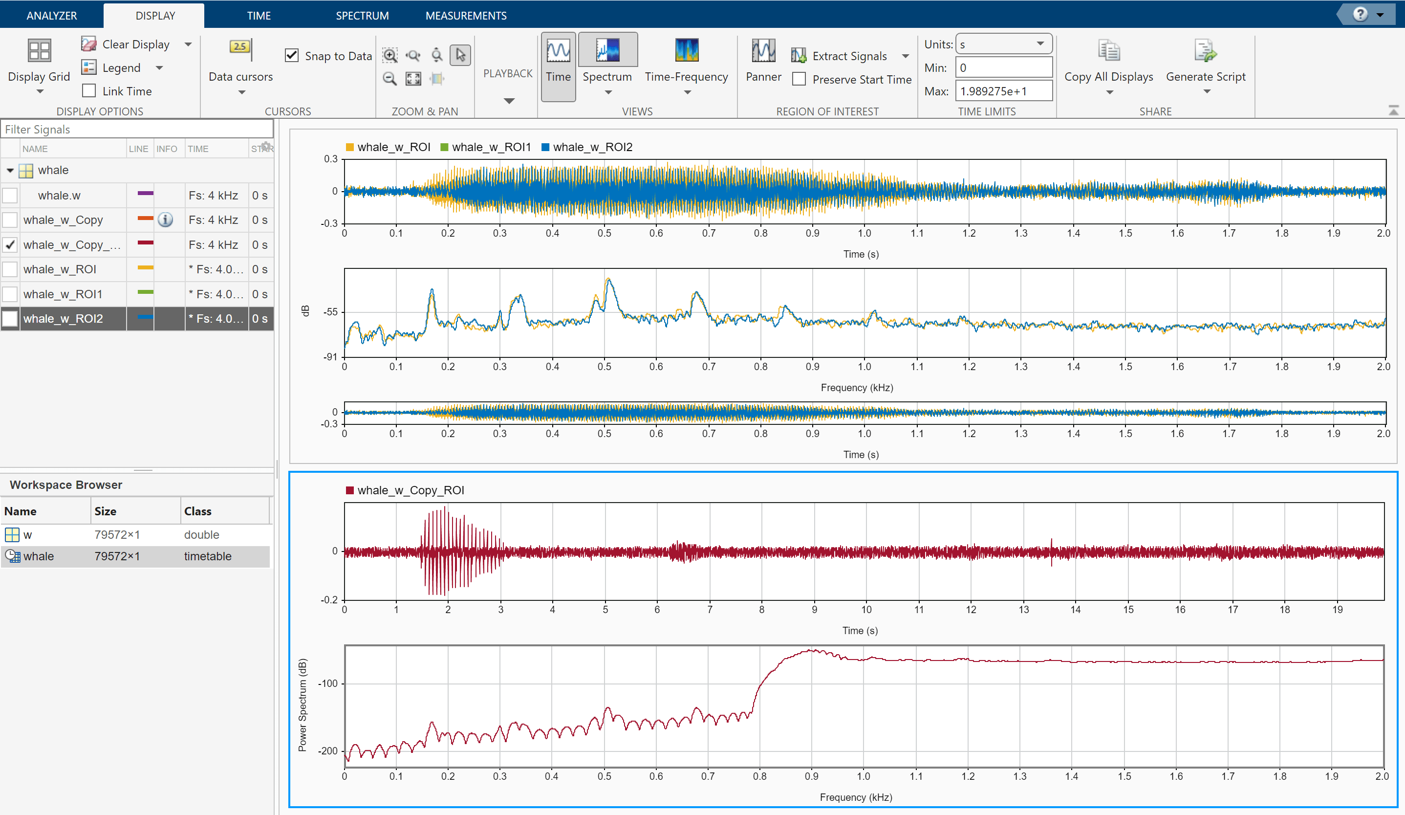
Remove the original signal from the display by clearing the check box next to its name in the Signal table. Display the three regions of interest you just extracted. Their spectra lie approximately on top of each other. Click Display Grid to add a second display and plot the region of interest containing the trill that you extracted and its spectrum. The trill and moan spectra are noticeably different.
Select the extracted signals in the Signal table. Click Export on the Analyzer tab to export the four regions of interest in a MAT-file.

See Also
Signal Analyzer | Signal Labeler
Related Topics
- Find Delay Between Correlated Signals
- Resolve Tones by Varying Window Leakage
- Find Interference Using Persistence Spectrum
- Modulation and Demodulation Using Complex Envelope
- Find and Track Ridges Using Reassigned Spectrogram
- Extract Voices from Music Signal
- Resample and Filter a Nonuniformly Sampled Signal
- Declip Saturated Signals Using Your Own Function
- Compute Envelope Spectrum of Vibration Signal
- Extract Regions of Interest from Whale Song
You can also select a web site from the following list:
Americas
- América Latina (Español)
- Canada (English)
- United States (English)
Europe
- Belgium (English)
- Denmark (English)
- Deutschland (Deutsch)
- España (Español)
- Finland (English)
- France (Français)
- Ireland (English)
- Italia (Italiano)
- Luxembourg (English)
- Netherlands (English)
- Norway (English)
- Österreich (Deutsch)
- Portugal (English)
- Sweden (English)
- Switzerland
- United Kingdom (English)