Choose a Wavelet
There are two types of wavelet analysis: continuous and multiresolution. The type of wavelet analysis best suited for your work depends on what you want to do with the data. This topic focuses on 1-D data, but you can apply the same principles to 2-D data. To learn how to perform and interpret each type of analysis, see Practical Introduction to Time-Frequency Analysis Using the Continuous Wavelet Transform and Practical Introduction to Multiresolution Analysis.
Time-Frequency Analysis
If your goal is to perform a detailed time-frequency analysis, choose the continuous wavelet transform (CWT). In terms of implementation, scales are discretized more finely in the CWT than in the discrete wavelet transform (DWT). For additional information, see Continuous and Discrete Wavelet Transforms.
Instantaneous Frequency
The CWT is superior to the short-time Fourier transform (STFT) for signals in which the instantaneous frequency grows rapidly. In the following figure, the instantaneous frequencies of the hyperbolic chirp are plotted as dashed lines in the spectrogram and CWT-derived scalogram. For additional information, see Time-Frequency Analysis and Continuous Wavelet Transform.

Localizing Transients
The CWT is good at localizing transients in nonstationary signals. In the following figure, observe how well the wavelet coefficients align with the abrupt changes that occur in the signal. For additional information, see Practical Introduction to Time-Frequency Analysis Using the Continuous Wavelet Transform.
![]()
Supported Wavelets
To obtain the continuous wavelet transform of your data, use cwt and cwtfilterbank. Both functions support the analytic wavelets listed in
the following table. By default, cwt and
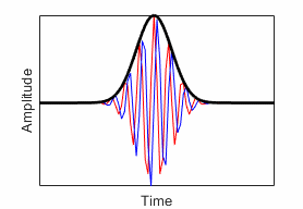
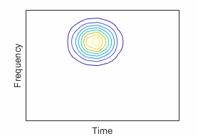
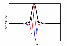
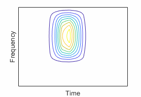
cwtfilterbank use the generalized Morse wavelet family. This
family is defined by two parameters. You can vary the parameters to recreate many
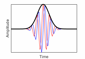
commonly used wavelets. In the time-domain plots, the red line and blue lines are
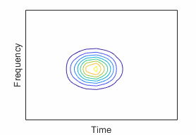
the real and imaginary parts, respectively, of the wavelet. The contour plots show
the wavelet spread in time and frequency. For additional information, see Morse Wavelets and Generalized Morse and Analytic Morlet Wavelets.
| Wavelet | Features | Name | Time Domain | Time-Frequency Domain |
|---|---|---|---|---|
| Generalized Morse Wavelet | Can vary two parameters to change time and frequency spread | "morse" (default) |
|
|
| Analytic Morlet (Gabor) Wavelet | Equal variance in time and frequency | "amor" |
|
|
| Bump Wavelet | Wider variance in time, narrower variance in frequency | "bump" |
|
|
All the wavelets in the table are analytic. Analytic wavelets are
wavelets with one-sided spectra and are complex valued in the time domain. These
wavelets are a good choice for obtaining a time-frequency analysis using the CWT.
Because the wavelet coefficients are complex valued, the CWT provides phase
information. cwt and cwtfilterbank support analytic and anti-analytic wavelets. For
additional information, see CWT-Based Time-Frequency Analysis.
Multiresolution Analysis
In a multiresolution analysis (MRA), you approximate a signal at progressively coarser
scales while recording the differences between approximations at consecutive scales. You
create the approximations and the differences by taking the discrete wavelet transform
(DWT) of the signal. The DWT provides a sparse representation for many natural signals.
Approximations are formed by comparing the signal with scaled and translated copies of a
scaling function. Differences between consecutive scales, also known as details, are
captured using scaled and translated copies of a wavelet. On a
log2 scale, the difference between
consecutive scales is always 1. In the case of the CWT, differences between consecutive
scales are finer.
When generating the MRA, you can either subsample (decimate) the approximation by a factor of 2 every time you increase the scale or not. Each option offers advantages and disadvantages. If you subsample, you end up with the same number of wavelet coefficients as the original signal. In the decimated DWT, translations are integer multiples of scale. For the nondecimated DWT, translations are integer shifts. A nondecimated DWT provides a redundant representation of the original data, but not as redundant as the CWT. Your application not only influences your choice of wavelet, but also which version of the DWT to use.
Energy Preservation
If preserving energy in the analysis stage is important, you must use an
orthogonal wavelet. An orthogonal transform preserves energy. Consider using an
orthogonal wavelet with compact support. Keep in mind that except for the Haar
wavelet, orthogonal wavelets with compact support are not symmetric. The associated
filters have nonlinear phase. This table lists supported orthogonal wavelets.
See
wavemngr("read") for all wavelet family names. To learn more
about a specific family, including wavelets available in that family, use waveinfo and the family short
name. For example, waveinfo("db").
| Orthogonal Wavelet Family (Family Short Name) | Features | Wavelet Name | See Also | Representative |
|---|---|---|---|---|
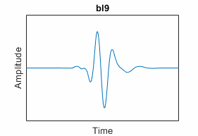
Best-localized Daubechies ("bl") | Compactly-supported wavelets similar to symlets; asymmetry of the symlets diminished in time by minimizing an additional second moment in time; scaling filter has N vanishing moments | "blN", where
N = 7, 9, and 10 | blscalf |
|
Beylkin ("beyl") | Has 18 coefficients and has 3 vanishing moments. | "beyl" |
| |
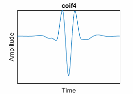
Coiflets ("coif") | Scaling function and wavelets have same number of vanishing moments N | "coifN", where
N = 1, 2, ..., 5 | coifwavf |
|
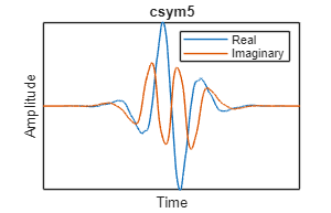
Complex Symlets
( | Complex-valued least asymmetric Daubechies wavelet; have the highest number of vanishing moments for a given support width; scaling filters have near-linear phase response and are symmetric for odd numbers of vanishing moments and least asymmetric for even numbers of vanishing moments. |
| csymwavf, daubfactors |
|
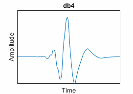
Daubechies ("db") | Extremal phase; energy concentrated near the start of their support; highest number of vanishing moments N for a given support width |
Note:
For N equal to 1, 2, and 3, the
| dbwavf,
daubfactors |
|
Fejér-Korovkin ("fk") | Filters constructed to minimize the difference between a valid scaling filter and the ideal sinc lowpass filter; filters have N coefficients, are especially useful in discrete (decimated and undecimated) wavelet packet transforms. | "fkN", where
N = 4, 6, 8, 14, 18, 22 | fejerkorovkin |
|
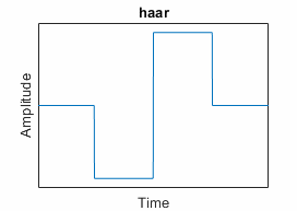
Haar ("haar") | Symmetric; special case of Daubechies; useful for edge detection | "haar", or equivalently,
"db1" |
| |
Han linear-phase moments ("han") | Characterized by a specified order of sum rules SR and order of linear-phase moments LP | "hanSR.LP";
to see supported values, use waveinfo and
the family short name | hanscalf |
|
Morris minimum-bandwidth ("mb") | Morris minimum-bandwidth orthogonal wavelets specified by the
number of filter coefficients (taps) N and
the level of the discrete wavelet transform L
used in the optimization; do not pass default orthogonality
checks in isorthwfb | "mbN.L";
to see supported values, use waveinfo and
the family short name | mbscalf |
|
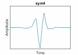
Symlets ("sym") | Least asymmetric; nearly linear phase; N vanishing moments |
Note:
For N equal to 1, 2, and 3, the
| symwavf,
daubfactors |
|
Vaidyanathan ("vaid") | Has 24 coefficients; does not pass default orthogonality
checks in isorthwfb | "vaid" |
|


Depending on how you address border distortions, the DWT might not conserve energy
in the analysis stage. For more information, see Border Effects. The maximal overlap discrete wavelet
transform modwt and maximal overlap discrete
wavelet packet transform modwpt do conserve energy. The
wavelet packet decomposition dwpt
does not conserve energy.
Feature Detection
If you want to find closely spaced features, choose wavelets with smaller support,
such as haar, db2, or sym2.
The support of the wavelet should be small enough to separate the features of
interest. Wavelets with larger support tend to have difficulty detecting closely
spaced features. Using wavelets with large support can result in coefficients that
do not distinguish individual features. In the following figure, the upper plot
shows a signal with spikes. The lower plot shows the first-level MRA details of a
maximal overlap DWT using the haar (thick blue lines) and
db6 (thick red lines) wavelets.

If your data has sparsely spaced transients, you can use wavelets with larger support.
Analysis of Variance
If your goal is to conduct an analysis of variance, the maximal overlap discrete wavelet transform (MODWT) is suited for the task. The MODWT is a variation of the standard DWT.
The MODWT conserves energy in the analysis stage.
The MODWT partitions variance across scales. For examples, see Wavelet Analysis of Financial Data and Wavelet Changepoint Detection.
The MODWT requires an orthogonal wavelet, such as a Daubechies wavelet or Symlet.
The MODWT is a shift-invariant transform. Shifting the input data shifts the wavelet coefficients by an identical amount. The decimated DWT is not shift invariant. Shifting the input changes the coefficients and can redistribute energy across scales.
See modwt, modwtmra, and modwtvar for more information. See
also Comparing MODWT and MODWTMRA.
Redundancy
Taking the decimated DWT, wavedec, of a signal using an
orthonormal family of wavelets provides a minimally redundant representation of the
signal. There is no overlap in wavelets within and across scales. The number of
coefficients equals the number of signal samples. Minimally redundant
representations are a good choice for compression, when you want to remove features
that are not perceived.
The CWT of a signal provides a highly redundant representation of a signal. There
is significant overlap between wavelets within and across scales. Also, given the
fine discretization of the scales, the cost to compute the CWT and store the wavelet
coefficients is significantly greater than the DWT. The MODWT modwt is also a redundant transform
but the redundancy factor is usually significantly less than the CWT. Redundancy
tends to reinforce signal characteristics and features you want to examine, such as
frequency breaks or other transient events.
If your work requires representing a signal with minimal redundancy, use wavedec. If your work requires a
redundant representation, use modwt or modwpt.
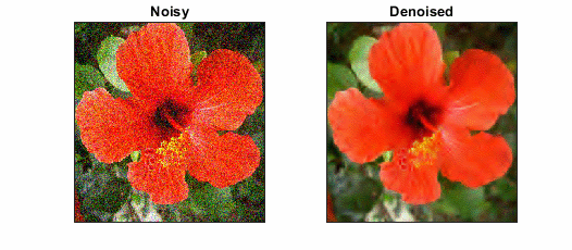
Denoising
An orthogonal wavelet, such as a Symlet or Daubechies wavelet, is a good choice for denoising signals. A biorthogonal wavelet can also be good for image processing. Biorthogonal wavelet filters have linear phase which is very critical for image processing. Using a biorthogonal wavelet will not introduce visual distortions in the image.
An orthogonal transform does not color white noise. If white noise is provided as input to an orthogonal transform, the output is white noise. Performing a DWT with a biorthogonal wavelet colors white noise.
An orthogonal transform preserves energy.
The sym4 wavelet is the default wavelet used in
wdenoise
and Wavelet Signal
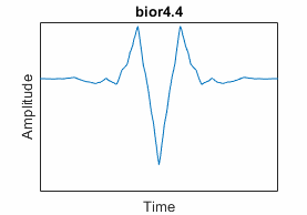
Denoiser app. The bior4.4 biorthogonal wavelet is the
default wavelet in wdenoise2.
Compression
If your work involves signal or image compression, consider using a biorthogonal wavelet. This table lists the supported biorthogonal wavelets with compact support.
| Biorthogonal Wavelet Family
(Family Short Name) | Features | Wavelet Name | Representative |
|---|---|---|---|
Biorthogonal Spline ("bior") | Compact support; symmetric filters; linear phase; specified by Nr and Nd, the number of vanishing moments for the reconstruction and decomposition filters respectively | "biorNr.Nd";
see waveinfo("bior") for supported values |
|
Reverse Biorthogonal Spline ("rbio") | Compact support; symmetric filters; linear phase; specified by Nr and Nd, the number of vanishing moments for the reconstruction and decomposition filters respectively | "rbioNd.Nr";
see waveinfo("rbio") for supported values |
|

Having two scaling function-wavelet pairs, one pair for analysis and another for synthesis, is useful for compression.
Biorthogonal wavelet filters are symmetric and have linear phase. (See Least Asymmetric Wavelet and Phase.)
The wavelets used for analysis can have many vanishing moments. A wavelet with N vanishing moments is orthogonal to polynomials of degree N-1. Using a wavelet with many vanishing moments results in fewer significant wavelet coefficients. Compression is improved.
The dual wavelets used for synthesis can have better regularity. The reconstructed signal is smoother.
Using an analysis filter with fewer vanishing moments than a synthesis filter can adversely affect compression. For an example, see Image Reconstruction with Biorthogonal Wavelets.
When using biorthogonal wavelets, energy is not conserved at the analysis stage. See Orthogonal and Biorthogonal Filter Banks for additional information.
General Considerations
Wavelets have properties that govern their behavior. Depending on what you want to do, some properties can be more important.
Orthogonality
If a wavelet is orthogonal, the wavelet transform preserves energy. Except for the Haar wavelet, no orthogonal wavelet with compact support is symmetric. The associated filter has nonlinear phase.
Vanishing Moments
A wavelet with N vanishing moments is orthogonal to polynomials of degree N−1. For an example, see Wavelets and Vanishing Moments. The number of vanishing moments and the oscillation of the wavelet have a loose relationship. As the number of vanishing moments grows, the greater the wavelet oscillates.
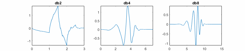
The number of vanishing moments also affects the support of a wavelet. Daubechies proved that a wavelet with N vanishing moments must have a support of at least length 2N-1.
Names for many wavelets are derived from the number of vanishing moments. For
example, db6 is the Daubechies wavelet with six vanishing
moments, and sym3 is the Symlet with three vanishing moments. For
coiflet wavelets, coif3 is the coiflet with six vanishing
moments. For Fejér-Korovkin wavelets, fk8 is the Fejér-Korovkin
wavelet with a length 8 filter. Biorthogonal wavelet names are derived from the
number of vanishing moments the analysis wavelet and synthesis wavelet each have.
For instance, bior3.5 is the biorthogonal wavelet with three
vanishing moments in the synthesis wavelet and five vanishing moments in the
analysis wavelet. To learn more, see waveinfo and wavemngr.
If the number of vanishing moments N is equal to 1, 2, or 3,
then dbN and
symN are identical.
Regularity
Regularity is related to how many continuous derivatives a function has. Intuitively, regularity can be considered a measure of smoothness. To detect an abrupt change in the data, a wavelet must be sufficiently regular. For a wavelet to have N continuous derivatives, the wavelet must have at least N+1 vanishing moments. See Detecting Discontinuities and Breakdown Points for an example. If your data is relatively smooth with few transients, a more regular wavelet might be a better fit for your work.
References
[1] Daubechies, Ingrid. Ten Lectures on Wavelets. Society for Industrial and Applied Mathematics, 1992.
[2] Morris, Joel M, and Ravindra Peravali. “Minimum-Bandwidth Discrete-Time Wavelets.” Signal Processing 76, no. 2 (July 1999): 181–93. https://doi.org/10.1016/S0165-1684(99)00007-9.
[3] Doroslovački, M.L. “On the Least Asymmetric Wavelets.” IEEE Transactions on Signal Processing 46, no. 4 (April 1998): 1125–30. https://doi.org/10.1109/78.668562.
[4] Han, Bin. “Wavelet Filter Banks.” In Framelets and Wavelets: Algorithms, Analysis, and Applications, 92–98. Applied and Numerical Harmonic Analysis. Cham, Switzerland: Birkhäuser, 2017. https://doi.org/10.1007/978-3-319-68530-4_2.
See Also
Apps
- Signal Multiresolution Analyzer | Wavelet Signal Analyzer | Wavelet Image Analyzer | Wavelet Signal Denoiser | Wavelet Time-Frequency Analyzer
Functions
cwt|cwtfilterbank|dwtfilterbank|wavedec|wavedec2|wdenoise2|wdenoise|waveinfo|wavemngr
Topics
- Practical Introduction to Multiresolution Analysis
- Practical Introduction to Time-Frequency Analysis Using the Continuous Wavelet Transform
- Understanding Wavelets, Part 1: What Are Wavelets
- Understanding Wavelets, Part 2: Types of Wavelet Transforms
- Understanding Wavelets, Part 3: An Example Application of the Discrete Wavelet Transform
- Understanding Wavelets, Part 4: An Example Application of the Continuous Wavelet Transform