sparss

Sparse first-order state-space model

Since R2020b

Description

Use sparss to represent sparse descriptor state-space models using matrices obtained from your finite element analysis (FEA) package. FEA involves the concept of dynamic substructuring where a mechanical system is partitioned into components that are modeled separately. These components are then coupled using rigid or semi-rigid physical interfaces that express consistency of displacements and equilibrium of internal forces. The resultant matrices from this type of modeling are quite large with a sparse pattern. Hence, using sparss is an efficient way to represent such large sparse state-space models in MATLAB^® to perform linear analysis. You can also use sparss to convert a second-order mechss model object to a sparss object.

You can use sparss model objects to represent SISO or MIMO state-space models in continuous time or discrete time. In continuous time, a first-order sparse state-space model is represented in the following form:

$\begin{array}{r} E \frac{d x}{d t} = A x (t) + B u (t) \\ y (t) = C x (t) + D u (t) \end{array}$

Here, x, u and y represent the states, inputs and outputs respectively, while A, B, C, D and E are the state-space matrices. The sparss object represents a state-space model in MATLAB storing sparse matrices A, B, C, D and E along with other information such as sample time, names and delays specific to the inputs and outputs.

You can use a sparss object to:

Perform time-domain and frequency-domain response analysis.
Specify signal-based connections with other LTI models.
Transform models between continuous-time and discrete-time representations.
Find low-order approximations of large sparse models.

For more information, see Sparse Model Basics.

Creation

Syntax

sys = sparss(A,B,C,D,E)

sys = sparss(A,B,C,D,E,ts)

sys = sparss(D)

sys = sparss(___,Name,Value)

sys = sparss(ltiSys)

Description

sys = sparss(A,B,C,D,E) creates a continuous-time first-order sparse state-space model object of the following form:

$\begin{array}{r} E \frac{d x}{d t} = A x (t) + B u (t) \\ y (t) = C x (t) + D u (t) \end{array}$

For instance, consider a plant with Nx states, Ny outputs, and Nu inputs. The first-order state-space matrices are:

A is the sparse state matrix with Nx-by-Nx real- or complex-values.
B is the sparse input-to-state matrix with Nx-by-Nu real- or complex-values.
is the sparse state-to-output matrix with Ny-by-Nx real- or complex-values.
D is the sparse gain or input-to-output matrix with Ny-by-Nu real- or complex-values.
E is the sparse mass matrix with the same size as matrix A. When E is omitted, sparss populates E with an identity matrix.

example

sys = sparss(A,B,C,D,E,ts) creates a discrete-time sparse state-space model with sample time ts with the form:

$\begin{array}{r} E x [k + 1] = A x [k] + B u [k] \\ y [k] = C x [k] + D u [k] \end{array}$

To leave the sample time unspecified, set ts to -1. When E is an identity matrix, you can set E as [] or omit E as long as A is not a scalar.

example

sys = sparss(D) creates a sparse state-space model that represents the static gain, D. The output state-space model is equivalent to sparss([],[],[],D,[]).

example

sys = sparss(___,Name,Value) sets properties of the first-order sparse state-space model using one or more name-value pair arguments. Use this syntax with any of the previous input-argument combinations.

example

sys = sparss(ltiSys) converts the dynamic system model ltiSys to a first-order sparse state-space model.

example

Input Arguments

expand all

`A` — State Matrix
`Nx`-by-`Nx` sparse matrix

State matrix, specified as an Nx-by-Nx sparse matrix, where Nx is the number of states. This input sets the value of property A.

`B` — Input-to-state matrix
`Nx`-by-`Nu` sparse matrix

Input-to-state matrix, specified as an Nx-by-Nu sparse matrix, where Nx is the number of states and Nu is the number of inputs. This input sets the value of property B.

`C` — State-to-output matrix
`Ny`-by-`Nx` sparse matrix

State-to-output matrix, specified as an Ny-by-Nx sparse matrix, where Nx is the number of states and Ny is the number of outputs. This input sets the value of property C.

`D` — Input-to-output matrix
`Ny`-by-`Nu` sparse matrix

Input-to-output matrix, specified as an Ny-by-Nu sparse matrix, where Ny is the number of outputs and Nu is the number of inputs. This input sets the value of property D.

`E` — Mass matrix
`Nx`-by-`Nx` sparse matrix

Mass matrix, specified as an Nx-by-Nx sparse matrix, where Nx is the number of states. This input sets the value of property E.

`ts` — Sample time
scalar

Sample time, specified as a scalar. For more information see the Ts property.

`ltiSys` — Dynamic system to convert to first-order sparse state-space form
dynamic system model | model array

Dynamic system to convert to first-order sparse state-space form, specified as a SISO or MIMO dynamic system model or array of dynamic system models. Dynamic systems that you can convert include:

Continuous-time or discrete-time numeric LTI models, such as mechss, tf, zpk, ss or pid models.

Output Arguments

expand all

`sys` — Output system model
`sparss` model object

Output system model, returned as a sparss model object.

Properties

expand all

`A` — State matrix
`Nx`-by-`Nx` sparse matrix

State matrix, specified as an Nx-by-Nx sparse matrix, where Nx is the number of states.

`B` — Input-to-state matrix
`Nx`-by-`Nu` sparse matrix

Input-to-state matrix, specified as an Nx-by-Nu sparse matrix, where Nx is the number of states and Nu is the number of inputs.

`C` — State-to-output matrix
`Ny`-by-`Nx` sparse matrix

State-to-output matrix, specified as an Ny-by-Nx sparse matrix, where Nx is the number of states and Ny is the number of outputs.

`D` — Input-to-output matrix
`Ny`-by-`Nu` sparse matrix

Input-to-output matrix, specified as an Ny-by-Nu sparse matrix, where Ny is the number of outputs and Nu is the number of inputs. D is also called as the static gain matrix which represents the ratio of the output to the input under steady state condition.

`E` — Mass matrix
`Nx`-by-`Nx` sparse matrix

Mass matrix, specified as a Nx-by-Nx sparse matrix. E is the same size as A.

Differential algebraic equations (DAEs) are characterized by their differential index, which is a measure of their singularity. A linear DAE is of index ≤1 if it can be transformed by congruence to the following form with E₁₁ and A₂₂ being invertible matrices.

$\begin{array}{r} E_{11} {\dot{x}}_{1} = A_{11} x_{1} + A_{12} x_{2} + B_{1} u \\ 0 = A_{21} x_{1} + A_{22} x_{2} + B_{2} u \end{array}$

The index of the DAE is 0 if x₂ is empty. The index is 1 if x₂ is not empty. In other words, a linear DAE has structural index ≤1 if it can be brought to the above form by row and column permutations of A and E. Some functionality, such as computing the impulse response of the system, is limited to DAEs with structural index less than 1.

For more information on DAE index, see Solve Differential Algebraic Equations (DAEs).

`Offsets` — Model offsets
`[]` (default) | structure

Since R2024a

Model offsets, specified as a structure with these fields.

Field	Description
`u`	Input offsets, specified as a vector of length equal to the number of inputs.
`y`	Output offsets, specified as a vector of length equal to the number of outputs.
`x`	State offsets, specified as a vector of length equal to the number of states.
`dx`	State derivative offsets, specified as a vector of length equal to the number of states.

For state-space model arrays, set Offsets to a structure array with the same dimension as the model array.

When you linearize the nonlinear model

$\begin{matrix} \dot{x} = f (x, u), & y = g (x, u) \end{matrix}$

around an operating point (x₀,u₀), the resulting model is a state-space model with offsets:

$\begin{matrix} \dot{x} = \underset{δ_{0}}{\underset{︸}{f (x_{0}, u_{0})}} + A (x - x_{0}) + B (u - u_{0}) \\ y = \underset{y_{0}}{\underset{︸}{g (x_{0}, u_{0})}} + C (x - x_{0}) + D (u - u_{0}), \end{matrix}$

where

$\begin{matrix} A = \frac{\partial f}{\partial x} (x_{0}, u_{0}), & B = \frac{\partial f}{\partial u} (x_{0}, u_{0}), & C = \frac{\partial g}{\partial x} (x_{0}, u_{0}), & D = \frac{\partial g}{\partial u} (x_{0}, u_{0}) . \end{matrix}$

For the linearization to be a good approximation of the nonlinear maps, it must include the offsets δ₀, x₀, u₀, and y₀. The linearize (Simulink Control Design) command returns both A, B, C, D and the offsets when using the StoreOffset option.

This property helps you manage linearization offsets and use them in operations such as response simulation, model interconnections, and model transformations.

`StateInfo` — State partition information
structure array

State partition information containing state vector components, interfaces between components and internal signal connecting components, specified as a structure array with the following fields:

Type — Type includes component, signal or physical interface
Name — Name of the component, signal or physical interface
Size — Number of states or degrees of freedom in the partition

You can view the partition information of the sparse state-space model using showStateInfo. You can also sort and order the partitions in your sparse model using xsort.

`SolverOptions` — Options for model analysis
structure

Options for model analysis, specified as a structure with the following fields:

UseParallel — Set this option true to enable parallel computing and false to disable it. Parallel computing is disabled by default. The UseParallel option requires a Parallel Computing Toolbox™ license.
DAESolver — Use this option to select the type of Differential Algebraic Equation (DAE) solver. The available DAE solvers are:
- 'trbdf2' — Fixed-step solver with an accuracy of o(h^2), where h is the step size.[1]
- 'trbdf3' — Fixed-step solver with an accuracy of o(h^3), where h is the step size.
Reducing the step size increases accuracy and extends the frequency range where numerical damping is negligible. 'trbdf3' is about 50% more computationally intensive than 'trbdf2'

`InternalDelay` — Internal delays in the model
vector

Internal delays in the model, specified as a vector. Internal delays arise, for example, when closing feedback loops on systems with delays, or when connecting delayed systems in series or parallel. For more information about internal delays, see Closing Feedback Loops with Time Delays.

For continuous-time models, internal delays are expressed in the time unit specified by the TimeUnit property of the model. For discrete-time models, internal delays are expressed as integer multiples of the sample time Ts. For example, InternalDelay = 3 means a delay of three sampling periods.

You can modify the values of internal delays using the property InternalDelay. However, the number of entries in sys.InternalDelay cannot change, because it is a structural property of the model.

`InputDelay` — Input delay
`0` (default) | scalar | `Nu`-by-1 vector

Input delay for each input channel, specified as one of the following:

Scalar — Specify the input delay for a SISO system or the same delay for all inputs of a multi-input system.
Nu-by-1 vector — Specify separate input delays for input of a multi-input system, where Nu is the number of inputs.

For continuous-time systems, specify input delays in the time unit specified by the TimeUnit property. For discrete-time systems, specify input delays in integer multiples of the sample time, Ts.

For more information, see Time Delays in Linear Systems.

`OutputDelay` — Output delay
`0` (default) | scalar | `Ny`-by-1 vector

Output delay for each output channel, specified as one of the following:

Scalar — Specify the output delay for a SISO system or the same delay for all outputs of a multi-output system.
Ny-by-1 vector — Specify separate output delays for output of a multi-output system, where Ny is the number of outputs.

For continuous-time systems, specify output delays in the time unit specified by the TimeUnit property. For discrete-time systems, specify output delays in integer multiples of the sample time, Ts.

For more information, see Time Delays in Linear Systems.

`Ts` — Sample time
`0` (default) | positive scalar | `-1`

Sample time, specified as:

0 for continuous-time systems.
A positive scalar representing the sampling period of a discrete-time system. Specify Ts in the time unit specified by the TimeUnit property.
-1 for a discrete-time system with an unspecified sample time.

Note

Changing Ts does not discretize or resample the model. To convert between continuous-time and discrete-time representations, use c2d and d2c. To change the sample time of a discrete-time system, use d2d.

`TimeUnit` — Time variable units
`'seconds'` (default) | `'nanoseconds'` | `'microseconds'` | `'milliseconds'` | `'minutes'` | `'hours'` | `'days'` | `'weeks'` | `'months'` | `'years'` | ...

Time variable units, specified as one of the following:

'nanoseconds'
'microseconds'
'milliseconds'
'seconds'
'minutes'
'hours'
'days'
'weeks'
'months'
'years'

Changing TimeUnit has no effect on other properties, but changes the overall system behavior. Use chgTimeUnit to convert between time units without modifying system behavior.

`InputName` — Input channel names
`''` (default) | character vector | cell array of character vectors

Input channel names, specified as one of the following:

A character vector, for single-input models.
A cell array of character vectors, for multi-input models.
'', no names specified, for any input channels.

Alternatively, you can assign input names for multi-input models using automatic vector expansion. For example, if sys is a two-input model, enter the following.

sys.InputName = 'controls';

The input names automatically expand to {'controls(1)';'controls(2)'}.

You can use the shorthand notation u to refer to the InputName property. For example, sys.u is equivalent to sys.InputName.

Use InputName to:

Identify channels on model display and plots.
Extract subsystems of MIMO systems.
Specify connection points when interconnecting models.

`InputUnit` — Input channel units
`''` (default) | character vector | cell array of character vectors

Input channel units, specified as one of the following:

A character vector, for single-input models.
A cell array of character vectors, for multi-input models.
'', no units specified, for any input channels.

Use InputUnit to specify input signal units. InputUnit has no effect on system behavior.

`InputGroup` — Input channel groups
structure

Input channel groups, specified as a structure. Use InputGroup to assign the input channels of MIMO systems into groups and refer to each group by name. The field names of InputGroup are the group names and the field values are the input channels of each group. For example, enter the following to create input groups named controls and noise that include input channels 1 and 2, and 3 and 5, respectively.

sys.InputGroup.controls = [1 2];
sys.InputGroup.noise = [3 5];

You can then extract the subsystem from the controls inputs to all outputs using the following.

sys(:,'controls')

By default, InputGroup is a structure with no fields.

`OutputName` — Output channel names
`''` (default) | character vector | cell array of character vectors

Output channel names, specified as one of the following:

A character vector, for single-output models.
A cell array of character vectors, for multi-output models.
'', no names specified, for any output channels.

Alternatively, you can assign output names for multi-output models using automatic vector expansion. For example, if sys is a two-output model, enter the following.

sys.OutputName = 'measurements';

The output names automatically expand to {'measurements(1)';'measurements(2)'}.

You can also use the shorthand notation y to refer to the OutputName property. For example, sys.y is equivalent to sys.OutputName.

Use OutputName to:

Identify channels on model display and plots.
Extract subsystems of MIMO systems.
Specify connection points when interconnecting models.

`OutputUnit` — Output channel units
`''` (default) | character vector | cell array of character vectors

Output channel units, specified as one of the following:

A character vector, for single-output models.
A cell array of character vectors, for multi-output models.
'', no units specified, for any output channels.

Use OutputUnit to specify output signal units. OutputUnit has no effect on system behavior.

`OutputGroup` — Output channel groups
structure

Output channel groups, specified as a structure. Use OutputGroup to assign the output channels of MIMO systems into groups and refer to each group by name. The field names of OutputGroup are the group names and the field values are the output channels of each group. For example, create output groups named temperature and measurement that include output channels 1, and 3 and 5, respectively.

sys.OutputGroup.temperature = [1];
sys.OutputGroup.measurement = [3 5];

You can then extract the subsystem from all inputs to the measurement outputs using the following.

sys('measurement',:)

By default, OutputGroup is a structure with no fields.

`Notes` — User-specified text
`{}` (default) | character vector | cell array of character vectors

User-specified text that you want to associate with the system, specified as a character vector or cell array of character vectors. For example, 'System is MIMO'.

`UserData` — User-specified data
`[]` (default) | any MATLAB data type

User-specified data that you want to associate with the system, specified as any MATLAB data type.

`Name` — System name
`''` (default) | character vector

System name, specified as a character vector. For example, 'system_1'.

`SamplingGrid` — Sampling grid for model arrays
structure array

Sampling grid for model arrays, specified as a structure array.

Use SamplingGrid to track the variable values associated with each model in a model array.

Set the field names of the structure to the names of the sampling variables. Set the field values to the sampled variable values associated with each model in the array. All sampling variables must be numeric scalars, and all arrays of sampled values must match the dimensions of the model array.

For example, you can create an 11-by-1 array of linear models, sysarr, by taking snapshots of a linear time-varying system at times t = 0:10. The following code stores the time samples with the linear models.

 sysarr.SamplingGrid = struct('time',0:10)

Similarly, you can create a 6-by-9 model array, M, by independently sampling two variables, zeta and w. The following code maps the (zeta,w) values to M.

[zeta,w] = ndgrid(<6 values of zeta>,<9 values of w>)
M.SamplingGrid = struct('zeta',zeta,'w',w)

By default, SamplingGrid is a structure with no fields.

Object Functions

The following lists show functions you can use with sparss model objects.

expand all

Modeling

`mechss`	Sparse second-order state-space model
`getx0`	Map initial conditions from a `mechss` object to a `sparss` object
`full`	Convert sparse models to dense storage
`imp2exp`	Convert implicit linear relationship to explicit input-output relation
`inv`	Invert dynamic system models
`getDelayModel`	State-space representation of internal delays

Data Access

`sparssdata`	Access first-order sparse state-space model data
`mechssdata`	Access second-order sparse state-space model data
`showStateInfo`	State vector map for sparse model
`spy`	Visualize sparsity pattern of a sparse model

Model Transformation

`c2d`	Convert model from continuous to discrete time
`d2c`	Convert model from discrete to continuous time
`d2d`	Resample discrete-time model

Time and Frequency Response

`step`	Step response of dynamic system
`impulse`	Impulse response plot of dynamic system; impulse response data
`initial`	System response to initial states of state-space model
`lsim`	Compute time response simulation data of dynamic system to arbitrary inputs
`bode`	Bode frequency response of dynamic system
`nyquist`	Nyquist response of dynamic system
`nichols`	Nichols response of dynamic system
`sigma`	Singular values of frequency response of dynamic system
`passiveplot`	Compute or plot passivity index as function of frequency
`dcgain`	Low-frequency (DC) gain of LTI system
`evalfr`	Evaluate system response at specific frequency
`freqresp`	Evaluate system response over a grid of frequencies

Model Interconnection

`interface`	Specify physical connections between components of `mechss` model
`xsort`	Sort states based on state partition
`feedback`	Feedback connection of multiple models
`parallel`	Parallel connection of two models
`append`	Group models by appending their inputs and outputs
`connect`	Block diagram interconnections of dynamic systems
`lft`	Generalized feedback interconnection of two models (Redheffer star product)
`series`	Series connection of two models

Examples

collapse all

Continuous-Time Sparse First-Order Model

Open Live Script

For this example, consider sparseFOContinuous.mat which contains sparse matrices for a continuous-time sparse first-order state-space model.

Extract the sparse matrices from sparseFOContinuous.mat.

load('sparseFOContinuous.mat','A','B','C','D','E');

Create the sparss model object.

sys = sparss(A,B,C,D,E)

Sparse continuous-time state-space model with 1 outputs, 1 inputs, and 199 states.

Use "spy" and "showStateInfo" to inspect model structure. 
Type "help sparssOptions" for available solver options for this model.

The output sys is a continuous-time sparss model object with 199 states, 1 input and 1 output.

You can use the spy command to visualize the sparsity of the sparss model object.

spy(sys)

Figure contains an axes object. The axes object with title nnz: A=239, E=239, B=20, C=19, D=1., xlabel Right-click to select matrices contains 7 objects of type line. One or more of the lines displays its values using only markers These objects represent A, B, C, D.

Discrete-Time Sparse First-Order Model

Open Live Script

For this example, consider sparseFODiscrete.mat which contains sparse matrices for a discrete-time sparse first-order state-space model.

Extract the sparse matrices from sparseFODiscrete.mat.

load('sparseFODiscrete.mat','A','B','C','D','E','ts');

Create the sparss model object.

sys = sparss(A,B,C,D,E,ts)

Sparse discrete-time state-space model with 1 outputs, 1 inputs, and 398 states.

Use "spy" and "showStateInfo" to inspect model structure. 
Type "help sparssOptions" for available solver options for this model.

The output sys is a discrete-time sparss model object with 398 states, 1 input and 1 output.

You can use the spy command to visualize the sparsity of the sparss model object.

spy(sys)

Figure contains an axes object. The axes object with title nnz: A=518, E=837, B=56, C=18, D=1., xlabel Right-click to select matrices contains 7 objects of type line. One or more of the lines displays its values using only markers These objects represent A, B, C, D.

You can also view model properties of the sparss model object.

properties('sparss')

Properties for class sparss:

    A
    B
    C
    D
    E
    Offsets
    Scaled
    StateInfo
    SolverOptions
    InternalDelay
    InputDelay
    OutputDelay
    InputName
    InputUnit
    InputGroup
    OutputName
    OutputUnit
    OutputGroup
    Notes
    UserData
    Name
    Ts
    TimeUnit
    SamplingGrid

MIMO Static Gain Sparse First-Order Model

Open Live Script

Create a static gain MIMO sparse first-order state-space model.

Consider the following three-input, two-output static gain matrix:

$D = [\begin{array}{ccc} 1 & 5 & 7 \\ 6 & 3 & 9 \end{array}]$

Specify the gain matrix and create the static gain sparse first-order state-space model.

D = [1,5,7;6,3,9];
sys = sparss(D);
size(sys)

Sparse state-space model with 2 outputs, 3 inputs, and 0 states.

Convert Second-Order Sparse Model to First-Order Sparse Model Representation

Open Live Script

For this example, consider mechssModel.mat that contains a mechss model object ltiSys.

Load the mechss model object from mechssModel.mat.

load('mechssModel.mat','ltiSys');
ltiSys

Sparse continuous-time second-order model with 1 outputs, 1 inputs, and 872 degrees of freedom.

Use "spy" and "showStateInfo" to inspect model structure. 
Type "help mechssOptions" for available solver options for this model.

Use the sparss command to convert to first-order sparse representation.

sys = sparss(ltiSys)

Sparse continuous-time state-space model with 1 outputs, 1 inputs, and 1744 states.

Use "spy" and "showStateInfo" to inspect model structure. 
Type "help sparssOptions" for available solver options for this model.

The resultant sparss model object sys has exactly double the number of states than the mechss object ltisys since the mass matrix M is full rank. If the mass matrix is not full rank then the number of states in the resultant sparss model when converting from a mechss model is between n and 2n. Here, n is the number of nodes in the mechss model object.

Sparse First-Order Model in a Feedback Loop

Open Live Script

For this example, consider sparseFOSignal.mat that contains a sparse first-order model. Define an actuator, sensor, and controller and connect them together with the plant in a feedback loop.

Load the sparse matrices and create the sparss object.

load sparseFOSignal.mat
plant = sparss(A,B,C,D,E,'Name','Plant');

Next, create an actuator and sensor using transfer functions.

act = tf(1,[1 2 3],'Name','Actuator');
sen = tf(1,[6 7],'Name','Sensor');

Create a PID controller object for the plant.

con = pid(1,1,0.1,0.01,'Name','Controller');

Use the feedback command to connect the plant, sensor, actuator, and controller in a feedback loop.

sys = feedback(sen*plant*act*con,1)

Sparse continuous-time state-space model with 1 outputs, 1 inputs, and 29 states.

Use "spy" and "showStateInfo" to inspect model structure. 
Type "help sparssOptions" for available solver options for this model.

The resultant system sys is a sparss object since sparss objects take precedence over tf and PID model object types.

Use showStateInfo to view the component and signal groups.

showStateInfo(sys)

The state groups are:

    Type          Name       Size
  -------------------------------
  Component      Sensor         1
  Component      Plant         20
  Signal                        1
  Component     Actuator        2
  Signal                        1
  Component    Controller       2
  Signal                        1
  Signal                        1

Use xsort to sort the components and signals, and then view the component and signal groups.

sysSort = xsort(sys);
showStateInfo(sysSort)

The state groups are:

    Type          Name       Size
  -------------------------------
  Component      Sensor         1
  Component      Plant         20
  Component     Actuator        2
  Component    Controller       2
  Signal                        4

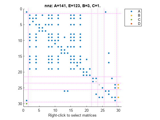
Observe that the components are now ordered before the signal partition. The signals are now sorted and grouped together in a single partition.

You can also visualize the sparsity pattern of the resultant system using spy.

spy(sysSort)

Figure contains an axes object. The axes object with title nnz: A=141, E=123, B=3, C=1., xlabel Right-click to select matrices contains 15 objects of type line. One or more of the lines displays its values using only markers These objects represent A, B, C, D.

References

[1] M. Hosea and L. Shampine. "Analysis and implementation of TR-BDF2." Applied Numerical Mathematics, vol. 20, no. 1-2, pp. 21-37, 1996.

Version History

Introduced in R2020b

expand all

R2024a: Create sparse state-space models with offsets

Use the new Offsets property to store model offsets. Offsets usually arise when linearizing nonlinear dynamics at some operating conditions. This property helps you manage linearization offsets and use them in operations such as response simulation, model interconnections, and model transformations.

sparss

Description

Creation

Syntax

Description

Input Arguments

A — State Matrix Nx-by-Nx sparse matrix

B — Input-to-state matrix Nx-by-Nu sparse matrix

C — State-to-output matrix Ny-by-Nx sparse matrix

D — Input-to-output matrix Ny-by-Nu sparse matrix

E — Mass matrix Nx-by-Nx sparse matrix

ts — Sample time scalar

ltiSys — Dynamic system to convert to first-order sparse state-space form dynamic system model | model array

Output Arguments

sys — Output system model sparss model object

Properties

A — State matrix Nx-by-Nx sparse matrix

B — Input-to-state matrix Nx-by-Nu sparse matrix

C — State-to-output matrix Ny-by-Nx sparse matrix

D — Input-to-output matrix Ny-by-Nu sparse matrix

E — Mass matrix Nx-by-Nx sparse matrix

Offsets — Model offsets [] (default) | structure

StateInfo — State partition information structure array

SolverOptions — Options for model analysis structure

InternalDelay — Internal delays in the model vector

InputDelay — Input delay 0 (default) | scalar | Nu-by-1 vector

OutputDelay — Output delay 0 (default) | scalar | Ny-by-1 vector

Ts — Sample time 0 (default) | positive scalar | -1

TimeUnit — Time variable units 'seconds' (default) | 'nanoseconds' | 'microseconds' | 'milliseconds' | 'minutes' | 'hours' | 'days' | 'weeks' | 'months' | 'years' | ...

InputName — Input channel names '' (default) | character vector | cell array of character vectors

InputUnit — Input channel units '' (default) | character vector | cell array of character vectors

InputGroup — Input channel groups structure

OutputName — Output channel names '' (default) | character vector | cell array of character vectors

OutputUnit — Output channel units '' (default) | character vector | cell array of character vectors

OutputGroup — Output channel groups structure

Notes — User-specified text {} (default) | character vector | cell array of character vectors

UserData — User-specified data [] (default) | any MATLAB data type

Name — System name '' (default) | character vector

SamplingGrid — Sampling grid for model arrays structure array

Object Functions

Modeling

Data Access

Model Transformation

Time and Frequency Response

Model Interconnection

Examples

Continuous-Time Sparse First-Order Model

Discrete-Time Sparse First-Order Model

MIMO Static Gain Sparse First-Order Model

Convert Second-Order Sparse Model to First-Order Sparse Model Representation

Sparse First-Order Model in a Feedback Loop

References

Version History

R2024a: Create sparse state-space models with offsets

See Also

Topics

`A` — State Matrix
`Nx`-by-`Nx` sparse matrix

`B` — Input-to-state matrix
`Nx`-by-`Nu` sparse matrix

`C` — State-to-output matrix
`Ny`-by-`Nx` sparse matrix

`D` — Input-to-output matrix
`Ny`-by-`Nu` sparse matrix

`E` — Mass matrix
`Nx`-by-`Nx` sparse matrix

`ts` — Sample time
scalar

`ltiSys` — Dynamic system to convert to first-order sparse state-space form
dynamic system model | model array

`sys` — Output system model
`sparss` model object

`A` — State matrix
`Nx`-by-`Nx` sparse matrix

`B` — Input-to-state matrix
`Nx`-by-`Nu` sparse matrix

`C` — State-to-output matrix
`Ny`-by-`Nx` sparse matrix

`D` — Input-to-output matrix
`Ny`-by-`Nu` sparse matrix

`E` — Mass matrix
`Nx`-by-`Nx` sparse matrix

`Offsets` — Model offsets
`[]` (default) | structure

`StateInfo` — State partition information
structure array

`SolverOptions` — Options for model analysis
structure

`InternalDelay` — Internal delays in the model
vector

`InputDelay` — Input delay
`0` (default) | scalar | `Nu`-by-1 vector

`OutputDelay` — Output delay
`0` (default) | scalar | `Ny`-by-1 vector

`Ts` — Sample time
`0` (default) | positive scalar | `-1`

`TimeUnit` — Time variable units
`'seconds'` (default) | `'nanoseconds'` | `'microseconds'` | `'milliseconds'` | `'minutes'` | `'hours'` | `'days'` | `'weeks'` | `'months'` | `'years'` | ...

`InputName` — Input channel names
`''` (default) | character vector | cell array of character vectors

`InputUnit` — Input channel units
`''` (default) | character vector | cell array of character vectors

`InputGroup` — Input channel groups
structure

`OutputName` — Output channel names
`''` (default) | character vector | cell array of character vectors

`OutputUnit` — Output channel units
`''` (default) | character vector | cell array of character vectors

`OutputGroup` — Output channel groups
structure

`Notes` — User-specified text
`{}` (default) | character vector | cell array of character vectors

`UserData` — User-specified data
`[]` (default) | any MATLAB data type

`Name` — System name
`''` (default) | character vector

`SamplingGrid` — Sampling grid for model arrays
structure array